Discrete Distributions

Overview

Discrete distributions describe the probability behavior of variables that can assume only a countable number of distinct values, typically non-negative integers (0, 1, 2, …). Unlike continuous distributions, discrete probability distributions assign probabilities to individual outcomes rather than ranges of values. They are fundamental to modeling real-world phenomena where outcomes are naturally discrete, such as counting events, success/failure scenarios, or categorical outcomes. Understanding discrete distributions is essential for statistical inference, hypothesis testing, and decision-making in fields ranging from quality control to epidemiology.

Key Characteristics and Applications: Discrete distributions are characterized by their probability mass function (PMF), which gives the probability of observing each possible value. Common real-world applications include modeling the number of defects in a manufacturing batch, the number of phone calls arriving at a call center, the outcome of coin flips or dice rolls, customer arrival patterns following a Poisson process, and the distribution of rare events. The choice of which discrete distribution to use depends on the underlying mechanism generating the data—whether it involves fixed numbers of independent trials, counting rare events, sampling without replacement, or other stochastic processes.

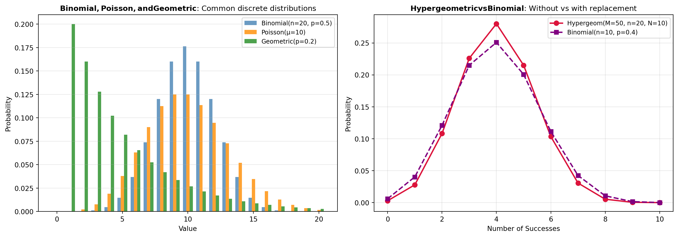
Fundamental Concepts: Several key concepts distinguish different discrete distributions. Bernoulli trials form the foundation for many discrete distributions, involving independent experiments with two outcomes (success or failure) with fixed probability. The binomial distribution, computed using tools like BINOM, results from the sum of independent Bernoulli trials and is used when you have a fixed number of trials with a constant success probability. The geometric distribution, accessed via GEOM, models the number of trials needed until the first success in a sequence of Bernoulli trials. The Poisson distribution, available through POISSON_DIST, models the number of events occurring in a fixed time interval when events happen at a constant average rate, making it ideal for rare events or arrival processes. The hypergeometric distribution, computed by HYPERGEOM, applies when sampling without replacement from a finite population with two categories.

Additional Specialized Distributions: Beyond the most common distributions, this category includes several specialized distributions for specific scenarios. The negative binomial distribution (NBINOM) generalizes the geometric distribution to model the number of trials until a fixed number of successes. The Zipf distribution (ZIPF) appears in many natural phenomena including word frequency in texts, city population rankings, and web traffic patterns, following a power-law relationship. The Yule-Simon distribution (YULESIMON) models similar power-law behaviors in evolutionary and linguistic contexts. The log-series distribution (LOGSER) describes abundance patterns in ecological data. The discrete Laplace distribution (DLAPLACE) provides a discrete analogue to the continuous Laplace distribution. Less common distributions like the beta-binomial (BETABINOM), beta-negative-binomial (BETANBINOM), negative hypergeometric (NHYPERGEOM), Boltzmann (BOLTZMANN), Planck (PLANCK), Skellam (SKELLAM), and Zipfian (ZIPFIAN) distributions serve specialized statistical and physical modeling needs.

Implementation Using SciPy: All discrete distributions in this category are implemented using SciPy’s scipy.stats module, which provides comprehensive functions for probability calculations. For each distribution, you can compute the probability mass function (PMF), giving the exact probability of discrete outcomes; the cumulative distribution function (CDF), showing the probability of observing a value less than or equal to a threshold; the survival function (SF), the complement of the CDF; the inverse CDF (ICDF) or quantile function, finding the value corresponding to a cumulative probability; the inverse SF (ISF); and distribution statistics including mean, variance, standard deviation, and median. This consistent interface across all distributions enables easy comparison and selection based on your data characteristics and modeling assumptions.

When to Use Each Distribution: The choice of distribution depends on your underlying data-generating mechanism. Use the binomial distribution when you have a fixed number of independent trials with constant success probability. Choose the Poisson distribution when modeling rare events or counts in a fixed time interval. Apply the hypergeometric distribution for sampling scenarios without replacement from finite populations. The geometric distribution is appropriate when measuring the number of trials until first success. The negative binomial distribution extends this to multiple successes. For categorical frequencies following power-law patterns, use Zipf or Yule-Simon distributions. When comparing two independent Poisson-distributed counts, the Skellam distribution is suitable. Specialized distributions like discrete Laplace, beta-binomial, and Planck address specific theoretical or applied contexts. Understanding the assumptions and constraints of each distribution ensures accurate statistical modeling and reliable inference.

Figure 1: Common discrete probability distributions: (A) Binomial, Poisson, and Geometric distributions showing different shapes based on parameters. (B) Comparison of Hypergeometric and Binomial distributions illustrating sampling with and without replacement.

Tools

Tool	Description
BERNOULLI	Calculates properties of a Bernoulli discrete random variable.
BETABINOM	Compute Beta-binomial distribution values from scipy.stats.betabinom.
BETANBINOM	Compute Beta-negative-binomial distribution values: PMF, CDF, SF, ICDF, ISF, mean, variance, std, or median.
BINOM	Compute Binomial distribution values: PMF, CDF, SF, ICDF, ISF, mean, variance, std, or median.
BOLTZMANN	Compute Boltzmann distribution values: PMF, CDF, SF, ICDF, ISF, mean, variance, std, or median.
DLAPLACE	Compute Discrete Laplace distribution values: PMF, CDF, SF, ICDF, ISF, mean, variance, std, or median.
GEOM	Compute Geometric distribution values using scipy.stats.geom.
HYPERGEOM	Compute Hypergeometric distribution values: PMF, CDF, SF, ICDF, ISF, mean, variance, std, or median.
LOGSER	Compute Log-Series distribution values: PMF, CDF, SF, ICDF, ISF, mean, variance, std, or median.
NBINOM	Compute Negative Binomial distribution values using scipy.stats.nbinom.
NHYPERGEOM	Compute Negative Hypergeometric distribution values using scipy.stats.nhypergeom.
PLANCK	Compute Planck distribution values using scipy.stats.planck.
POISSON_DIST	Compute Poisson distribution values using scipy.stats.poisson.
RANDINT	Compute Uniform discrete distribution values: PMF, CDF, SF, ICDF, ISF, mean, variance, std, or median.
SKELLAM	Compute Skellam distribution values using scipy.stats.skellam.
YULESIMON	Compute Yule-Simon distribution values using scipy.stats.yulesimon.
ZIPF	Compute Zipf distribution values: PMF, CDF, SF, ICDF, ISF, mean, variance, std, or median.
ZIPFIAN	Compute Zipfian distribution values: PMF, CDF, SF, ICDF, ISF, mean, variance, std, or median.