Count Models
Overview
Count data models are regression techniques designed for dependent variables that take non-negative integer values: 0, 1, 2, 3, and so forth. These models address a fundamental challenge in statistical modeling where traditional ordinary least squares regression is inappropriate. Count data arises naturally in numerous applied contexts: healthcare studies measuring the number of doctor visits or hospital admissions, insurance analytics tracking accident claims or insurance claims frequency, manufacturing quality control counting defects per unit, ecology monitoring species abundance, and epidemiology examining disease incident counts. Unlike continuous variables that can take any real value, count data has inherent discreteness and non-negativity constraints that require specialized statistical approaches.
The foundational model for count data is Poisson regression, which assumes that the count follows a Poisson distribution with mean parameter λ. However, real-world count data frequently violates the critical equidispersion assumption—that the mean equals the variance. In fact, most empirical count data exhibits overdispersion, where the variance substantially exceeds the mean, invalidating Poisson model confidence intervals and standard errors. Additionally, empirical count distributions often contain excess zeros—far more observations with zero counts than the Poisson distribution would predict. A dataset measuring doctor visits might have 30% zeros from healthy individuals, but Poisson predicts only 5%. These twin challenges of overdispersion and excess zeros motivate more sophisticated count models.
Implementation: These tools leverage Statsmodels for count data regression, with support from NumPy and SciPy for numerical optimization and statistical inference. Statsmodels provides robust implementations of advanced count models with automatic maximum likelihood estimation, hypothesis testing, and goodness-of-fit diagnostics.
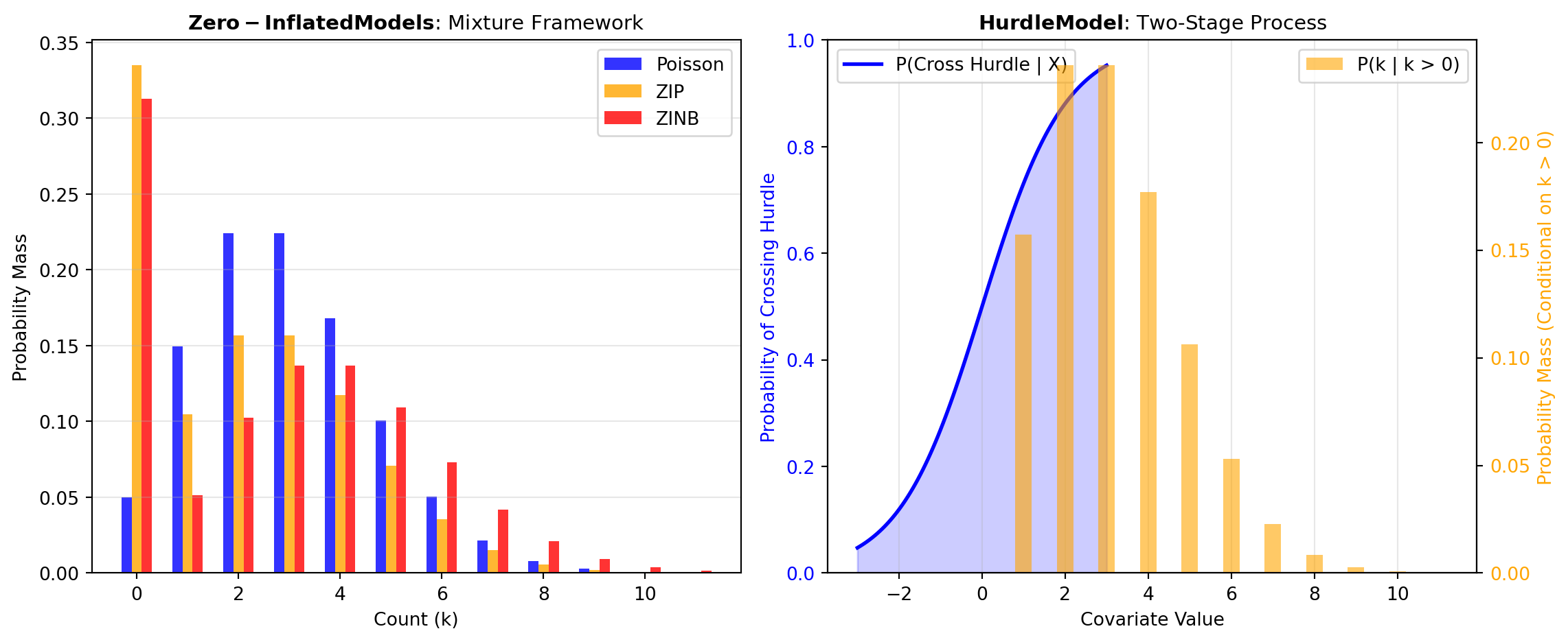
Zero-Inflated Models: The most common approach to excess zeros uses a mixture model framework that combines two probabilistic processes. The ZIP_MODEL implements Zero-Inflated Poisson regression, which models a split population: some individuals are in a “zero state” (structural zeros, always counted as zero) while others follow a Poisson process with positive probability of any count. This two-component structure naturally accommodates populations with inherently different zero-generation mechanisms. For example, in dental visit data, one component represents people who avoid dentists entirely, while another component represents regular dental patients following a Poisson count process. ZIP models are ideal when you expect a mixture of truly non-users and active users, with the probability of being in each component estimated from observed covariates.
The ZINB_MODEL extends zero-inflated concepts to handle both excess zeros and overdispersion simultaneously by replacing the Poisson component with a Negative Binomial distribution. The Negative Binomial accommodates variance far exceeding the mean through an additional dispersion parameter, providing substantially more modeling flexibility. ZINB is appropriate when your data exhibits both a substantial excess of zeros and strong variance-mean inequality, making it one of the most flexible count models for real-world applications.
Two-Stage Models: An alternative framework uses sequential decision-making processes where the data generation occurs in distinct stages. The HURDLE_COUNT_MODEL models a binary hurdle decision (will any count occur?) followed by a counting process for the magnitude conditional on crossing the hurdle. Unlike zero-inflated models that blend two populations, hurdle models use a true two-stage process: first, a logistic model determines the probability of any activity occurring; second, conditional on activity occurring, a truncated count model determines the magnitude. This structure suits scenarios with structural distinction between decisions to engage and decisions about engagement intensity—such as labor supply decisions (do you work?) followed by hours worked conditional on employment.
Figure 1 compares how these three major approaches characterize the relationship between covariates and the count outcome through different mechanisms: excess zeros and their origin, dispersion structure, and model flexibility. Selection among these tools depends on the specific data characteristics, research questions about zero-generation, and whether inference about the binary decision differs fundamentally from inference about the count magnitude.
Tools
| Tool | Description |
|---|---|
| HURDLE_COUNT_MODEL | Fits a Hurdle model for count data with two-stage process (zero vs. |
| ZINB_MODEL | Fits a Zero-Inflated Negative Binomial (ZINB) model for overdispersed count data with excess zeros. |
| ZIP_MODEL | Fits a Zero-Inflated Poisson (ZIP) model for count data with excess zeros. |