Models
Overview
Statistical models are mathematical frameworks that represent how data is generated, enabling us to estimate relationships between variables, make predictions, and understand underlying mechanisms. Unlike simple summary statistics, models can account for confounding factors, quantify uncertainty, and test hypotheses about complex processes. This category encompasses a broad range of modeling approaches from basic linear regression to advanced mixed-effects and survival models.
Foundation and Purpose
At their core, statistical models specify assumptions about how observed data relates to unobserved parameters. The process typically involves specifying a probability model, choosing appropriate estimation methods, and assessing model fit. Python implementations of statistical models primarily rely on statsmodels, which provides a comprehensive suite of modeling tools, alongside NumPy for numerical computation and SciPy for statistical functions.
Regression Models
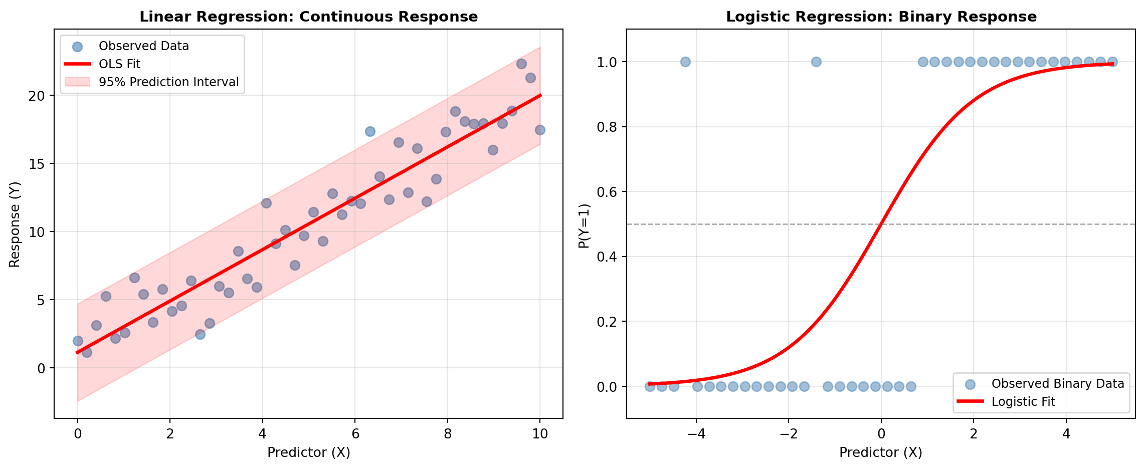
The Regression subcategory includes linear models that form the foundation of statistical inference. Ordinary Least Squares (OLS) regression minimizes squared deviations between observed and predicted values, suitable for continuous outcomes with approximately normal errors. Weighted Least Squares (WLS) and Generalized Least Squares (GLS) extend OLS to handle heteroscedasticity and correlation structures. Quantile regression models relationships at different points of the conditional distribution, useful when the effect of predictors varies across quantiles. Beyond standard linear models, robust regression uses M-estimators that downweight outliers, and specification tests help identify model misspecification before relying on results.
Generalized Linear Models
The Generalized Linear subcategory extends linear models to non-normal response distributions through link functions. Generalized Linear Models (GLM) with different families—binomial for binary/proportion data, Poisson for counts, Gamma for positive right-skewed data, Negative Binomial for overdispersed counts, and Tweedie for flexible distribution modeling—allow flexible modeling of various data types. These models use maximum likelihood estimation and are fundamental for handling outcomes beyond continuous normally-distributed responses.
Discrete Choice Models
When the response is categorical, the Discrete Choice subcategory provides specialized approaches. Logistic regression models binary outcomes, multinomial logit extends this to multiple unordered categories, ordered logit respects ordinal structure in categorical outcomes, and probit models offer an alternative parameterization using the normal cumulative distribution function. These models are essential for classification problems and understanding how predictors influence categorical choices.
Count Data Models
The Count subcategory addresses challenges in modeling non-negative integer responses. Standard Poisson models assume the mean equals the variance, but data often exhibits overdispersion (variance exceeds mean) or excess zeros. Zero-Inflated Poisson (ZIP) and Zero-Inflated Negative Binomial (ZINB) models accommodate excess zeros through mixture processes. Hurdle models explicitly separate the process determining whether a count is zero from the distribution of positive counts, providing interpretable two-stage modeling.
Mixed Effects Models
Clustered or hierarchical data requires accounting for within-group correlation. The Mixed Effects subcategory includes Linear Mixed Models (LMM) with random intercepts and slopes for continuous outcomes, Generalized Linear Mixed Models (GLMM) extending GLM to hierarchical structures with binomial or Poisson families, and Generalized Estimating Equations (GEE) for population-averaged inference in correlated data. These approaches simultaneously model fixed population effects and random subject-specific deviations.
Survival Analysis
The Survival subcategory handles time-to-event data with censoring. Kaplan-Meier estimators provide non-parametric survival function estimates by time group. Cox Proportional Hazards models extend this to regression by modeling how covariates affect the instantaneous risk of events while making minimal distributional assumptions. Parametric survival models (e.g., exponential) assume specific distributions and are useful when proportionality assumptions are questionable.
MEDIATION_ANALYSIS
This function estimates mediation effects to quantify how much of the relationship between a predictor and an outcome is explained through one or more mediator variables.
The total effect of predictor X on outcome Y is decomposed into a direct effect and an indirect effect through mediator M:
c = c' + ab
where c is the total effect, c' is the direct effect, and ab is the indirect effect. Confidence intervals and p-values for indirect effects are estimated using non-parametric bootstrap resampling.
Input data is provided as an Excel range where the first row contains column names and subsequent rows contain observations.
Excel Usage
=MEDIATION_ANALYSIS(data, x, m, y, covar, alpha, n_boot, seed)data(list[list], required): Input table as a 2D range with header row followed by observation rows.x(str, required): Predictor column name.m(str, required): Mediator column name, or comma-separated mediator column names for parallel mediation.y(str, required): Outcome column name.covar(str, optional, default: null): Optional covariate column name, or comma-separated covariate names.alpha(float, optional, default: 0.05): Significance level for confidence intervals (unitless).n_boot(int, optional, default: 500): Number of bootstrap resamples used for indirect effect inference.seed(int, optional, default: null): Optional random seed for reproducible bootstrap sampling.
Returns (list[list]): Mediation summary table with path coefficients, uncertainty metrics, confidence intervals, p-values, and significance labels.
Example 1: Single mediator with deterministic linear trend
Inputs:
| data | x | m | y | alpha | n_boot | seed | ||
|---|---|---|---|---|---|---|---|---|
| X | M | Y | X | M | Y | 0.05 | 200 | 42 |
| 1 | 2.2 | 2.3 | ||||||
| 2 | 2.8 | 3.1 | ||||||
| 3 | 3.9 | 4.3 | ||||||
| 4 | 5 | 5.2 | ||||||
| 5 | 5.9 | 6 | ||||||
| 6 | 7.1 | 7.4 | ||||||
| 7 | 8.2 | 8 | ||||||
| 8 | 8.8 | 9.2 | ||||||
| 9 | 9.9 | 10.1 | ||||||
| 10 | 11.1 | 11.4 |
Excel formula:
=MEDIATION_ANALYSIS({"X","M","Y";1,2.2,2.3;2,2.8,3.1;3,3.9,4.3;4,5,5.2;5,5.9,6;6,7.1,7.4;7,8.2,8;8,8.8,9.2;9,9.9,10.1;10,11.1,11.4}, "X", "M", "Y", 0.05, 200, 42)Expected output:
| path | coef | se | pval | CI2.5 | CI97.5 | sig |
|---|---|---|---|---|---|---|
| M ~ X | 1.00061 | 0.0177938 | 1.10999e-11 | 0.959573 | 1.04164 | Yes |
| Y ~ M | 0.998804 | 0.0208822 | 4.03763e-11 | 0.95065 | 1.04696 | Yes |
| Total | 1.00121 | 0.0174025 | 9.24967e-12 | 0.961082 | 1.04134 | Yes |
| Direct | 0.714205 | 0.354058 | 0.0834744 | -0.123008 | 1.55142 | No |
| Indirect | 0.287007 | 0.521284 | 0.47 | -0.47981 | 1.01255 | No |
Example 2: Single mediator with one covariate
Inputs:
| data | x | m | y | covar | alpha | n_boot | seed | |||
|---|---|---|---|---|---|---|---|---|---|---|
| X | M | Y | C | X | M | Y | C | 0.05 | 200 | 7 |
| 1 | 2.2 | 2.3 | 0 | |||||||
| 2 | 2.8 | 3.1 | 1 | |||||||
| 3 | 3.9 | 4.3 | 0 | |||||||
| 4 | 5 | 5.2 | 1 | |||||||
| 5 | 5.9 | 6 | 0 | |||||||
| 6 | 7.1 | 7.4 | 1 | |||||||
| 7 | 8.2 | 8 | 0 | |||||||
| 8 | 8.8 | 9.2 | 1 | |||||||
| 9 | 9.9 | 10.1 | 0 | |||||||
| 10 | 11.1 | 11.4 | 1 |
Excel formula:
=MEDIATION_ANALYSIS({"X","M","Y","C";1,2.2,2.3,0;2,2.8,3.1,1;3,3.9,4.3,0;4,5,5.2,1;5,5.9,6,0;6,7.1,7.4,1;7,8.2,8,0;8,8.8,9.2,1;9,9.9,10.1,0;10,11.1,11.4,1}, "X", "M", "Y", "C", 0.05, 200, 7)Expected output:
| path | coef | se | pval | CI2.5 | CI97.5 | sig |
|---|---|---|---|---|---|---|
| M ~ X | 1.0025 | 0.0188746 | 2.19775e-10 | 0.957869 | 1.04713 | Yes |
| Y ~ M | 0.993524 | 0.0190439 | 2.49089e-10 | 0.948492 | 1.03856 | Yes |
| Total | 0.9975 | 0.017087 | 1.13571e-10 | 0.957096 | 1.0379 | Yes |
| Direct | 0.603033 | 0.334092 | 0.121113 | -0.214461 | 1.42053 | No |
| Indirect | 0.394467 | 0.408463 | 0.36 | -0.266288 | 1.49213 | No |
Example 3: Two parallel mediators using comma-separated names
Inputs:
| data | x | m | y | alpha | n_boot | seed | |||
|---|---|---|---|---|---|---|---|---|---|
| X | M | Mtwo | Y | X | M, Mtwo | Y | 0.05 | 150 | 5 |
| 1 | 2.2 | 0.3 | 2.3 | ||||||
| 2 | 2.8 | 0.4 | 3.1 | ||||||
| 3 | 3.9 | 0.8 | 4.3 | ||||||
| 4 | 5 | 1 | 5.2 | ||||||
| 5 | 5.9 | 1.4 | 6 | ||||||
| 6 | 7.1 | 1.8 | 7.4 | ||||||
| 7 | 8.2 | 2.2 | 8 | ||||||
| 8 | 8.8 | 2.4 | 9.2 | ||||||
| 9 | 9.9 | 2.7 | 10.1 | ||||||
| 10 | 11.1 | 3.2 | 11.4 |
Excel formula:
=MEDIATION_ANALYSIS({"X","M","Mtwo","Y";1,2.2,0.3,2.3;2,2.8,0.4,3.1;3,3.9,0.8,4.3;4,5,1,5.2;5,5.9,1.4,6;6,7.1,1.8,7.4;7,8.2,2.2,8;8,8.8,2.4,9.2;9,9.9,2.7,10.1;10,11.1,3.2,11.4}, "X", "M, Mtwo", "Y", 0.05, 150, 5)Expected output:
| path | coef | se | pval | CI2.5 | CI97.5 | sig |
|---|---|---|---|---|---|---|
| M ~ X | 1.00061 | 0.0177938 | 1.10999e-11 | 0.959573 | 1.04164 | Yes |
| Mtwo ~ X | 0.328485 | 0.0105931 | 1.27149e-9 | 0.304057 | 0.352913 | Yes |
| Y ~ M | 0.99363 | 0.363678 | 0.029247 | 0.133667 | 1.85359 | Yes |
| Y ~ Mtwo | 0.0157464 | 1.10462 | 0.989024 | -2.59628 | 2.62777 | No |
| Total | 1.00121 | 0.0174025 | 9.24967e-12 | 0.961082 | 1.04134 | Yes |
| Direct | 0.798207 | 0.389274 | 0.0861822 | -0.154312 | 1.75073 | No |
| Indirect M | -0.0106336 | 1.3718 | 0.946667 | -3.21739 | 1.24809 | No |
| Indirect Mtwo | 0.213639 | 0.766531 | 0.426667 | -0.191389 | 2.34114 | No |
Example 4: Different alpha and bootstrap size
Inputs:
| data | x | m | y | alpha | n_boot | seed | ||
|---|---|---|---|---|---|---|---|---|
| X | M | Y | X | M | Y | 0.1 | 120 | 11 |
| 1 | 2.2 | 2.3 | ||||||
| 2 | 2.8 | 3.1 | ||||||
| 3 | 3.9 | 4.3 | ||||||
| 4 | 5 | 5.2 | ||||||
| 5 | 5.9 | 6 | ||||||
| 6 | 7.1 | 7.4 | ||||||
| 7 | 8.2 | 8 | ||||||
| 8 | 8.8 | 9.2 | ||||||
| 9 | 9.9 | 10.1 | ||||||
| 10 | 11.1 | 11.4 |
Excel formula:
=MEDIATION_ANALYSIS({"X","M","Y";1,2.2,2.3;2,2.8,3.1;3,3.9,4.3;4,5,5.2;5,5.9,6;6,7.1,7.4;7,8.2,8;8,8.8,9.2;9,9.9,10.1;10,11.1,11.4}, "X", "M", "Y", 0.1, 120, 11)Expected output:
| path | coef | se | pval | CI5.0 | CI95.0 | sig |
|---|---|---|---|---|---|---|
| M ~ X | 1.00061 | 0.0177938 | 1.10999e-11 | 0.967518 | 1.03369 | Yes |
| Y ~ M | 0.998804 | 0.0208822 | 4.03763e-11 | 0.959973 | 1.03764 | Yes |
| Total | 1.00121 | 0.0174025 | 9.24967e-12 | 0.968851 | 1.03357 | Yes |
| Direct | 0.714205 | 0.354058 | 0.0834744 | 0.0434153 | 1.385 | Yes |
| Indirect | 0.287007 | 0.405663 | 0.433333 | -0.244521 | 1.01084 | No |
Python Code
Show Code
import pandas as pd
import pingouin as pg

def mediation_analysis(data, x, m, y, covar=None, alpha=0.05, n_boot=500, seed=None):
    """
    Perform causal mediation analysis with bootstrap confidence intervals.

    See: https://pingouin-stats.org/generated/pingouin.mediation_analysis.html

    This example function is provided as-is without any representation of accuracy.

    Args:
        data (list[list]): Input table as a 2D range with header row followed by observation rows.
        x (str): Predictor column name.
        m (str): Mediator column name, or comma-separated mediator column names for parallel mediation.
        y (str): Outcome column name.
        covar (str, optional): Optional covariate column name, or comma-separated covariate names. Default is None.
        alpha (float, optional): Significance level for confidence intervals (unitless). Default is 0.05.
        n_boot (int, optional): Number of bootstrap resamples used for indirect effect inference. Default is 500.
        seed (int, optional): Optional random seed for reproducible bootstrap sampling. Default is None.

    Returns:
        list[list]: Mediation summary table with path coefficients, uncertainty metrics, confidence intervals, p-values, and significance labels.
    """
    try:
        def to2d(x):
            return [[x]] if not isinstance(x, list) else x

        def parse_names(value):
            if value is None:
                return None
            text = str(value).strip()
            if text == "":
                return None
            names = [part.strip() for part in text.split(",") if part.strip()]
            if len(names) == 0:
                return None
            return names

        matrix = to2d(data)
        if not isinstance(matrix, list) or len(matrix) < 2 or not all(isinstance(row, list) for row in matrix):
            return "Error: Invalid input - data must be a 2D list with a header row and at least one data row"

        header = [str(col).strip() for col in matrix[0]]
        if len(header) == 0 or any(col == "" for col in header):
            return "Error: Invalid input - header row must contain non-empty column names"

        width = len(header)
        rows = []
        for row in matrix[1:]:
            row_values = list(row)
            if len(row_values) < width:
                row_values = row_values + [None] * (width - len(row_values))
            elif len(row_values) > width:
                row_values = row_values[:width]
            rows.append(row_values)

        if len(rows) == 0:
            return "Error: Invalid input - at least one observation row is required"

        frame = pd.DataFrame(rows, columns=header)

        m_list = parse_names(m)
        if m_list is None:
            return "Error: Invalid input - m must contain at least one mediator column name"
        m_arg = m_list[0] if len(m_list) == 1 else m_list

        covar_list = parse_names(covar)
        covar_arg = None if covar_list is None else (covar_list[0] if len(covar_list) == 1 else covar_list)

        seed_arg = None if seed is None else int(seed)

        stats = pg.mediation_analysis(
            data=frame,
            x=str(x),
            m=m_arg,
            y=str(y),
            covar=covar_arg,
            alpha=float(alpha),
            n_boot=int(n_boot),
            seed=seed_arg,
            return_dist=False,
        )

        columns = [str(col) for col in stats.columns.tolist()]
        output = [columns]
        for row in stats.itertuples(index=False, name=None):
            out_row = []
            for value in row:
                if pd.isna(value):
                    out_row.append("")
                else:
                    out_row.append(value)
            output.append(out_row)

        max_len = max(len(r) for r in output)
        return [r + [""] * (max_len - len(r)) for r in output]
    except Exception as e:
        return f"Error: {str(e)}"
Online Calculator
Input table as a 2D range with header row followed by observation rows.
Predictor column name.
Mediator column name, or comma-separated mediator column names for parallel mediation.
Outcome column name.
Optional covariate column name, or comma-separated covariate names.
Significance level for confidence intervals (unitless).
Number of bootstrap resamples used for indirect effect inference.
Optional random seed for reproducible bootstrap sampling.