Curve Fitting
Overview
Curve fitting is the process of constructing a mathematical function that best approximates a series of data points. At its heart, curve fitting transforms empirical observations into predictive models, enabling interpolation, extrapolation, and scientific insight. The fundamental question is deceptively simple: given a set of (x, y) pairs, what function f(x) best captures the underlying relationship?
This discipline bridges theory and experiment across virtually every quantitative field. In chemistry and biochemistry, curve fitting extracts kinetic parameters from reaction rates and binding assays. In engineering, it models system responses, material properties, and signal characteristics. In economics and finance, it reveals trends, cycles, and forecast trajectories. The ubiquity of curve fitting reflects a deeper truth: real-world phenomena rarely present themselves as clean equations—we must infer them from noisy, incomplete data.
Mathematical Foundation
Curve fitting fundamentally addresses the problem of finding parameters \theta = (\theta_1, \theta_2, \ldots, \theta_p) for a model function f(x; \theta) such that it best represents the relationship between independent variables x and observed data y. The “best” representation is typically defined by minimizing a cost function, most commonly the sum of squared residuals: \text{SSR} = \sum_{i=1}^{n} (y_i - f(x_i; \theta))^2
This approach, known as least squares fitting, has dominated the field since its formulation by Gauss and Legendre. It provides both computational efficiency and useful statistical properties—assuming normally distributed errors, least squares estimation yields maximum likelihood estimates.
More generally, curve fitting involves choosing a parametric model, which explicitly specifies the functional form (linear, polynomial, exponential, logistic, etc.), and then solving an optimization problem to find parameter values that minimize the discrepancy between model predictions and observations. This is fundamentally different from non-parametric approaches like interpolation, where we construct a function passing through or near data points without assuming a specific mathematical form.
Implementation with Python
Modern curve fitting in Python relies on several powerful libraries that handle both standard models and arbitrary user-defined functions. SciPy, the foundational scientific computing library, provides scipy.optimize.curve_fit, a robust implementation of the Levenberg-Marquardt algorithm—a widely-used method that interpolates between gradient descent and the Gauss-Newton method. NumPy underpins all numerical operations and provides polynomial fitting via numpy.polyfit for the special case of polynomial models.
For more advanced applications, lmfit extends SciPy’s capabilities with built-in models, easy parameter constraints, and comprehensive uncertainty analysis through covariance matrix estimation. iminuit offers an alternative minimization framework based on Minuit (the algorithm engine behind CERN’s ROOT framework), providing automatic differentiation and sophisticated uncertainty propagation. For symbolic and automatic differentiation approaches, CasADi enables fitting arbitrary expressions with full gradient and Hessian computation.
Key Concepts and Approaches
Least Squares Fitting remains the dominant approach because it combines interpretability, computational efficiency, and statistical soundness. When errors are normally distributed with constant variance, least squares estimates are optimal in the sense of maximum likelihood. Tools like CURVE_FIT, LM_FIT, MINUIT_FIT, and CA_CURVE_FIT all implement variations of this principle, differing in algorithm selection, constraint handling, and uncertainty estimation methods.
Model Selection is the art of choosing which functional form to fit. The same data can be approximated by many different functions—polynomials, exponentials, power laws, sigmoid curves, and specialized domain-specific models. Empirical models (like DOSE_RESPONSE, ENZYME_BASIC, and GROWTH_SIGMOID) encode scientific knowledge about how systems behave in particular domains. Generic models like polynomials and exponentials provide flexibility but less physical insight.
Uncertainty Quantification answers the question: how confident are we in the fitted parameters? Least squares fitting naturally provides standard errors and confidence intervals through the covariance matrix of the fitted parameters. Tools like MINUIT_FIT and LM_FIT automatically compute these quantities, whereas CURVE_FIT requires explicit covariance calculation.
Regularization and Constraints become important when fitting ill-posed or underdetermined problems. Many tools allow bounds on parameters (e.g., requiring positive values for rate constants) or soft constraints that penalize unrealistic parameter combinations. This is essential in scientific applications where parameters have physical interpretations and must satisfy known constraints.
Specialized Models dominate practical applications. When you have domain knowledge—whether modeling enzyme kinetics, adsorption isotherms, chromatography peaks, or growth curves—using a specialized model class like BINDING_MODEL, ADSORPTION, or CHROMA_PEAKS ensures the fitted parameters have scientific meaning and improves convergence reliability.
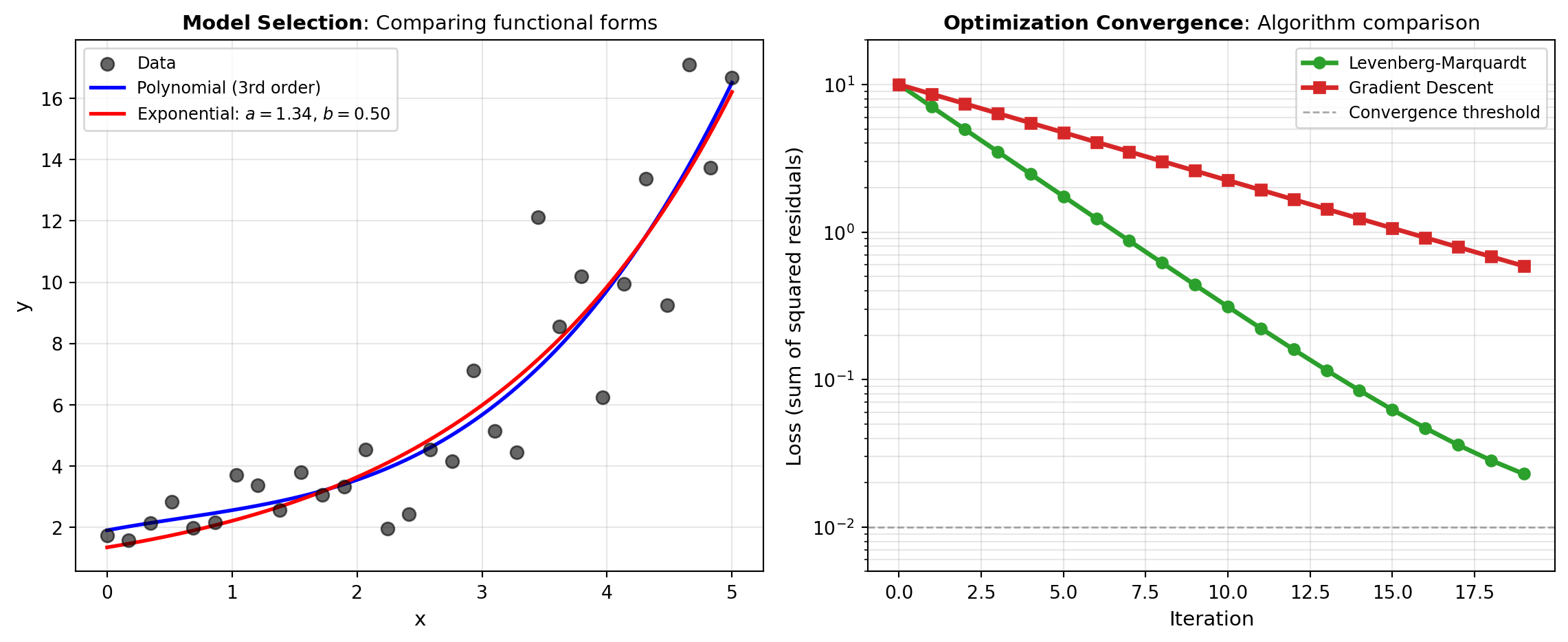
The visualization below illustrates two fundamental curve fitting scenarios: least squares fitting of synthetic data to both polynomial and exponential models, and the comparison of different optimization algorithms converging to the optimal parameter values.
Least Squares
| Tool | Description |
|---|---|
| CA_CURVE_FIT | Fit an arbitrary symbolic model to data using CasADi and automatic differentiation. |
| CURVE_FIT | Fit a model expression to xdata, ydata using scipy.optimize.curve_fit. |
| LM_FIT | Fit data using lmfit’s built-in models with optional model composition. |
| MINUIT_FIT | Fit an arbitrary model expression to data using iminuit least-squares minimization with uncertainty estimates. |
Models
| Tool | Description |
|---|---|
| ADSORPTION | Fits adsorption models to data using scipy.optimize.curve_fit. |
| AGRICULTURE | Fits agriculture models to data using scipy.optimize.curve_fit. |
| BINDING_MODEL | Fits binding_model models to data using scipy.optimize.curve_fit. |
| CHROMA_PEAKS | Fits chroma_peaks models to data using scipy.optimize.curve_fit. |
| DOSE_RESPONSE | Fits dose_response models to data using scipy.optimize.curve_fit. |
| ELECTRO_ION | Fits electro_ion models to data using scipy.optimize.curve_fit. |
| ENZYME_BASIC | Fits enzyme_basic models to data using scipy.optimize.curve_fit. |
| ENZYME_INHIBIT | Fits enzyme_inhibit models to data using scipy.optimize.curve_fit. |
| EXP_ADVANCED | Fits exp_advanced models to data using scipy.optimize.curve_fit. |
| EXP_DECAY | Fits exp_decay models to data using scipy.optimize.curve_fit. |
| EXP_GROWTH | Fits exponential growth models to data using scipy.optimize.curve_fit. |
| GROWTH_POWER | Fits growth_power models to data using scipy.optimize.curve_fit. |
| GROWTH_SIGMOID | Fits growth_sigmoid models to data using scipy.optimize.curve_fit. |
| MISC_PIECEWISE | Fits misc_piecewise models to data using scipy.optimize.curve_fit. |
| PEAK_ASYM | Fits peak_asym models to data using scipy.optimize.curve_fit. |
| POLY_BASIC | Fits poly_basic models to data using scipy.optimize.curve_fit. |
| RHEOLOGY | Fits rheology models to data using scipy.optimize.curve_fit. |
| SPECTRO_PEAKS | Fits spectro_peaks models to data using scipy.optimize.curve_fit. |
| STAT_DISTRIB | Fits stat_distrib models to data using scipy.optimize.curve_fit. |
| STAT_PARETO | Fits stat_pareto models to data using scipy.optimize.curve_fit. |
| WAVEFORM | Fits waveform models to data using scipy.optimize.curve_fit. |