Continuous Distributions

Overview

Continuous probability distributions describe variables that can take any value within a range, encompassing measurements like time, temperature, weight, distance, and financial returns. Unlike discrete distributions that assign probabilities to individual points, continuous distributions define probability densities over intervals—the probability of observing any single exact value is zero, but probabilities are well-defined for regions.

Continuous distributions form the mathematical foundation for statistical inference, hypothesis testing, and modeling real-world phenomena. They arise naturally whenever measurements are made on continuous scales or when we model aggregate effects of many small independent factors (via the Central Limit Theorem). Understanding the shapes, tails, and moments of continuous distributions enables researchers to choose appropriate models for their data and to conduct valid statistical analyses.

Background and Applications: Continuous distributions serve critical roles across domains. In quality control, the normal distribution models manufacturing variations. In reliability engineering, the Weibull distribution describes equipment failure times. In financial modeling, distributions like the lognormal characterize asset returns and price movements. In Bayesian statistics, distributions like the beta and uniform act as prior distributions, encoding prior beliefs about parameters. In hypothesis testing, distributions like Student’s t and the chi-squared distribution determine critical values and p-values.

Implementation: These tools leverage SciPy, specifically the scipy.stats module, which provides comprehensive implementations of continuous distributions along with methods for probability density functions (PDFs), cumulative distribution functions (CDFs), quantile functions (inverse CDFs), random sampling, and distribution statistics. This enables seamless integration with NumPy for numerical computation and vectorized operations.

Key Probability Concepts: Every continuous distribution has fundamental properties that characterize its behavior. The probability density function (PDF) describes the relative likelihood of values; the area under the PDF over an interval gives the probability of that interval. The cumulative distribution function (CDF) gives the probability of being less than or equal to a specific value—monotonically increasing from 0 to 1. The quantile function (inverse CDF) answers the reverse question: what value corresponds to a given cumulative probability? The survival function gives the probability of exceeding a value, complementary to the CDF.

Distribution Families: Several fundamental families of continuous distributions address different modeling needs. The NORM (normal/Gaussian) distribution is symmetric and ubiquitous due to the Central Limit Theorem; use it for modeling sums of independent effects and as a default for approximately symmetric data. The EXPON (exponential) distribution models waiting times and inter-arrival intervals with a constant hazard rate; it’s memoryless, making it ideal for processes without aging. The UNIFORM distribution represents complete uncertainty within bounds; use it when all values in a range are equally likely or as a reference distribution.

Shape Variation and Flexibility: Beyond simple families, flexible distributions adapt to diverse data shapes. The BETA distribution spans 0 to 1 with adjustable shape parameters, making it ideal for proportions and probabilities; it also serves as a conjugate prior in Bayesian analysis. The WEIBULL_MIN distribution generalizes the exponential with adjustable hazard rates (increasing, constant, or decreasing); use it for reliability modeling and survival analysis where failure rates vary over time. The LOGNORM distribution models right-skewed positive data; apply it to income distributions, particle sizes, and multiplicative processes.

Tail Behavior and Extremes: Different distributions exhibit different tail characteristics crucial for extreme value analysis. The PARETO distribution has heavy, power-law tails modeling phenomena like wealth distribution and firm sizes. The CAUCHY distribution has extremely heavy tails with undefined mean and variance; it arises in physics (resonance phenomena) but presents challenges for standard statistical methods. The T_DIST (Student’s t) distribution has heavier tails than normal, accounting for uncertainty in sample-based estimation; use it in t-tests and when constructing confidence intervals with small samples.

Specialized Distributions: Certain distributions address specific analytical needs. The CHISQ distribution emerges in goodness-of-fit testing and is related to chi-squared tests for independence. The F_DIST distribution arises in comparing variances and appears in analysis of variance (ANOVA). The LAPLACE distribution combines exponential tails symmetrically, useful for robust regression and modeling double-exponential phenomena.

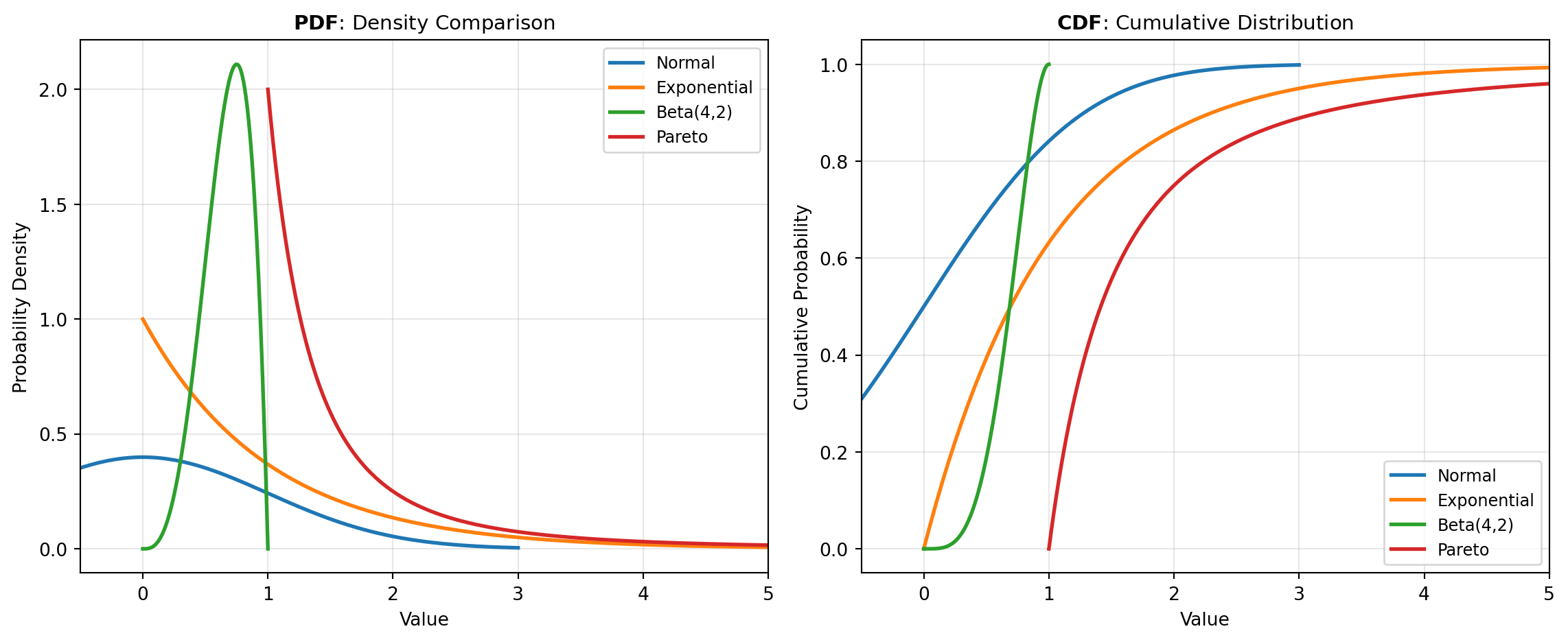
Figure Figure 1 visualizes how several key distributions compare in their probability density and their cumulative probabilities, illustrating the diverse shapes available for modeling.

Figure 1: Continuous Distribution Characteristics: (A) Probability density functions (PDFs) comparing normal, exponential, beta, and Pareto distributions, showing symmetric, right-skewed, flexible, and heavy-tailed behaviors. (B) Cumulative distribution functions (CDFs) for the same distributions, illustrating how probability accumulates and displaying tail behavior differences.

Tools

Tool	Description
BETA	Wrapper for scipy.stats.beta distribution providing multiple statistical methods.
CAUCHY	Wrapper for scipy.stats.cauchy distribution providing multiple statistical methods.
CHISQ	Compute various statistics and functions for the chi-squared distribution from scipy.stats.chi2.
EXPON	Exponential distribution function wrapping scipy.stats.expon.
F_DIST	Unified interface to the main methods of the F-distribution, including PDF, CDF, inverse CDF, survival function, and distribution statistics.
LAPLACE	Laplace distribution function supporting multiple methods.
LOGNORM	Compute lognormal distribution statistics and evaluations.
NORM	Normal (Gaussian) distribution function supporting multiple methods.
PARETO	Generalized Pareto distribution function supporting multiple methods.
T_DIST	Student’s t distribution function supporting multiple methods from scipy.stats.t.
UNIFORM	Uniform distribution function supporting multiple methods.
WEIBULL_MIN	Compute various functions of the Weibull minimum distribution using scipy.stats.weibull_min.