Hypothesis Tests
Overview
Hypothesis testing is a formal statistical procedure used to determine whether an observed effect in data is real or likely due to random chance. It provides a structured framework for making evidence-based decisions about populations based on sample data. All hypothesis tests in this category are implemented using SciPy’s comprehensive statistical functions.
Fundamental Concepts
Every hypothesis test involves setting up competing claims about a population parameter:
- Null Hypothesis (H_0): The default assumption that there is no effect or no difference (e.g., “There is no difference between the groups” or “The variable has no association”).
- Alternative Hypothesis (H_1 or H_a): The claim you are testing for (e.g., “Group A differs from Group B” or “The variables are associated”).
- P-value: The probability of observing results as extreme as or more extreme than those obtained, assuming the null hypothesis is true. When p < \alpha (typically 0.05), we reject H_0 in favor of H_1.
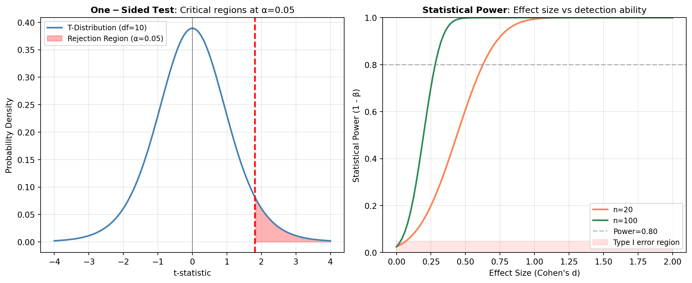
- Significance Level (\alpha): The threshold (usually 0.05) for deciding whether the p-value provides sufficient evidence against the null hypothesis.
- Type I and Type II Errors: Type I (false positive) occurs when rejecting a true H_0; Type II (false negative) occurs when failing to reject a false H_0.
Test Selection by Data Structure
Hypothesis tests are organized by the structure of your data and research question:
One Sample Tests: Used when testing a single sample against a population parameter or theoretical distribution. These include tests for the mean (e.g.,
TTEST_1SAMP), goodness-of-fit tests (e.g.,SHAPIRO,KSTEST), and tests for specific distributional properties (e.g.,NORMALTESTfor normality,JARQUE_BERAfor skewness and kurtosis).Independent Sample Tests: Used when comparing two or more independent groups or samples. These range from parametric tests assuming normality and equal variances (e.g.,
TTEST_IND,F_ONEWAY) to non-parametric alternatives (e.g.,MANNWHITNEYU,KRUSKAL) and specialized tests for variance equality (e.g.,LEVENE,FLIGNER) and multiple comparison corrections (e.g.,DUNNETT).Association and Correlation Tests: Used when examining relationships between two or more variables. These include correlation-based tests (e.g.,
PEARSONR,SPEARMANR,KENDALLTAU) for measuring linear or monotonic associations, tests of independence for categorical variables (e.g.,CHI2_CONTINGENCY,FISHER_EXACT), and robust regression alternatives (e.g.,THEILSLOPES,SIEGELSLOPES) for estimating relationships while reducing the influence of outliers.
Choosing the Right Test
Choosing Between Paired and Independent T-Tests
One of the most frequent decisions in hypothesis testing is whether to use a paired or independent t-test. The choice depends entirely on how your samples are related.
| Feature | Independent T-test | Paired T-test |
|---|---|---|
| Comparison | Two different groups (e.g., Treatment A vs. Treatment B) | The same group at two times (e.g., Before vs. After) |
| Sample Size | Can be different | Must be equal |
| Dependency | Samples are unrelated | Each value in X matches exactly one value in Y |
| Statistical Power | Lower (more noise) | Higher (controls for individual variation) |
[!TIP] Implementation Note: To perform a paired t-test using Boardflare tools, calculate the difference between your paired observations (D = X - Y) and run a One-Sample T-test on those differences with a null hypothesis of H_0: \mu_D = 0.
Python Example: Paired vs. Independent
import numpy as np
from scipy import stats

# 1. Independent data
group_a = [85, 92, 78, 88, 90]
group_b = [72, 80, 68, 75, 82]
result_ind = stats.ttest_ind(group_a, group_b)

# 2. Paired data (before/after)
before = [85, 92, 78, 88, 90]
after  = [88, 95, 80, 90, 95]
diff = np.array(after) - np.array(before)

# Paired test is equivalent to 1-sample test on differences
result_paired = stats.ttest_rel(before, after)
result_1samp = stats.ttest_1samp(diff, 0)

print(f"Independent p-value: {result_ind.pvalue:.4f}")
print(f"Paired p-value:      {result_paired.pvalue:.4f}")
print(f"1-Sample p-value:    {result_1samp.pvalue:.4f} (equivalent to paired)")
Your choice of test depends on several factors: the number of samples or groups, whether your data are independent or paired, the scale of measurement (continuous, ordinal, categorical), whether you want to assume normality and equal variances, and your research hypothesis (one-sided or two-sided). Parametric tests are generally more powerful when their assumptions are met, while non-parametric tests are more robust to violations of these assumptions but may have less power. Exact tests (e.g., FISHER_EXACT, BARNARD_EXACT) are particularly useful for small sample sizes or sparse contingency tables.
ANOVA
One-way analysis of variance tests whether group means are equal across levels of a categorical factor.
The test compares between-group variability to within-group variability through the F statistic:
F = \frac{\text{MS}_{\text{between}}}{\text{MS}_{\text{within}}}
This wrapper accepts a table with headers, selects the dependent variable and grouping column, and returns the ANOVA table produced by Pingouin.
Excel Usage
=ANOVA(data, dv, between, ss_type, detailed, effsize)data(list[list], required): Input table where the first row contains column names.dv(str, required): Name of the dependent-variable column.between(str, required): Name of the between-subject factor column.ss_type(int, optional, default: 2): Sum-of-squares type (typically 1, 2, or 3).detailed(bool, optional, default: false): Whether to return a detailed ANOVA table.effsize(str, optional, default: “np2”): Effect size metric (for example, np2, n2, ng2).
Returns (list[list]): 2D table containing the ANOVA results.
Example 1: Balanced one-way design with three groups
Inputs:
| data | dv | between | |
|---|---|---|---|
| score | group | score | group |
| 5.1 | A | ||
| 5.4 | A | ||
| 6.3 | B | ||
| 6.5 | B | ||
| 7 | C | ||
| 7.2 | C |
Excel formula:
=ANOVA({"score","group";5.1,"A";5.4,"A";6.3,"B";6.5,"B";7,"C";7.2,"C"}, "score", "group")Expected output:
| Source | ddof1 | ddof2 | F | p_unc | np2 |
|---|---|---|---|---|---|
| group | 2 | 3 | 61.5882 | 0.00366618 | 0.976224 |
Example 2: Detailed table enabled
Inputs:
| data | dv | between | detailed | |
|---|---|---|---|---|
| score | group | score | group | true |
| 10 | X | |||
| 11 | X | |||
| 9 | X | |||
| 14 | Y | |||
| 15 | Y | |||
| 16 | Y |
Excel formula:
=ANOVA({"score","group";10,"X";11,"X";9,"X";14,"Y";15,"Y";16,"Y"}, "score", "group", TRUE)Expected output:
| Source | SS | DF | MS | F | p_unc | np2 |
|---|---|---|---|---|---|---|
| group | 37.5 | 1 | 37.5 | 37.5 | 0.00360223 | 0.903614 |
| Within | 4 | 4 | 1 |
Example 3: Sum-of-squares type three
Inputs:
| data | dv | between | ss_type | |
|---|---|---|---|---|
| score | group | score | group | 3 |
| 2.1 | G1 | |||
| 2.2 | G1 | |||
| 3 | G2 | |||
| 3.1 | G2 | |||
| 4.2 | G3 | |||
| 4.4 | G3 |
Excel formula:
=ANOVA({"score","group";2.1,"G1";2.2,"G1";3,"G2";3.1,"G2";4.2,"G3";4.4,"G3"}, "score", "group", 3)Expected output:
| Source | ddof1 | ddof2 | F | p_unc | np2 |
|---|---|---|---|---|---|
| group | 2 | 3 | 233.167 | 0.000511046 | 0.993608 |
Example 4: Alternate effect size metric
Inputs:
| data | dv | between | effsize | |
|---|---|---|---|---|
| outcome | condition | outcome | condition | n2 |
| 1.2 | C1 | |||
| 1.4 | C1 | |||
| 2 | C2 | |||
| 2.2 | C2 | |||
| 2.9 | C3 | |||
| 3.1 | C3 |
Excel formula:
=ANOVA({"outcome","condition";1.2,"C1";1.4,"C1";2,"C2";2.2,"C2";2.9,"C3";3.1,"C3"}, "outcome", "condition", "n2")Expected output:
| Source | ddof1 | ddof2 | F | p_unc | n2 |
|---|---|---|---|---|---|
| condition | 2 | 3 | 72.3333 | 0.00289573 | 0.979684 |
Python Code
Show Code
import pandas as pd
from pingouin import anova as pg_anova

def anova(data, dv, between, ss_type=2, detailed=False, effsize='np2'):
    """
    Perform one-way ANOVA on tabular data using Pingouin.

    See: https://pingouin-stats.org/build/html/generated/pingouin.anova.html

    This example function is provided as-is without any representation of accuracy.

    Args:
        data (list[list]): Input table where the first row contains column names.
        dv (str): Name of the dependent-variable column.
        between (str): Name of the between-subject factor column.
        ss_type (int, optional): Sum-of-squares type (typically 1, 2, or 3). Default is 2.
        detailed (bool, optional): Whether to return a detailed ANOVA table. Default is False.
        effsize (str, optional): Effect size metric (for example, np2, n2, ng2). Default is 'np2'.

    Returns:
        list[list]: 2D table containing the ANOVA results.
    """
    try:
        def to2d(x):
            return [[x]] if not isinstance(x, list) else x

        def build_dataframe(table):
            table = to2d(table)
            if not isinstance(table, list) or not table or not all(isinstance(row, list) for row in table):
                return None, "Error: data must be a non-empty 2D list"
            if len(table) < 2:
                return None, "Error: data must include a header row and at least one data row"

            headers = [str(h).strip() for h in table[0]]
            if not headers or any(h == "" for h in headers):
                return None, "Error: header row contains empty column names"
            if len(set(headers)) != len(headers):
                return None, "Error: header row contains duplicate column names"

            rows = []
            for row in table[1:]:
                if len(row) != len(headers):
                    return None, "Error: all data rows must match header width"
                rows.append([None if cell == "" else cell for cell in row])

            return pd.DataFrame(rows, columns=headers), None

        def dataframe_to_2d(df):
            out = [list(df.columns)]
            for values in df.itertuples(index=False, name=None):
                row = []
                for value in values:
                    if pd.isna(value):
                        row.append("")
                    elif isinstance(value, bool):
                        row.append(value)
                    elif isinstance(value, (int, float)):
                        row.append(float(value))
                    else:
                        row.append(str(value))
                out.append(row)
            return out

        frame, error = build_dataframe(data)
        if error:
            return error

        if dv not in frame.columns:
            return f"Error: dv column '{dv}' not found"
        if between not in frame.columns:
            return f"Error: between column '{between}' not found"

        result = pg_anova(
            data=frame,
            dv=dv,
            between=between,
            ss_type=int(ss_type),
            detailed=bool(detailed),
            effsize=effsize,
        )

        return dataframe_to_2d(result)
    except Exception as e:
        return f"Error: {str(e)}"
Online Calculator
Input table where the first row contains column names.
Name of the dependent-variable column.
Name of the between-subject factor column.
Sum-of-squares type (typically 1, 2, or 3).
Whether to return a detailed ANOVA table.
Effect size metric (for example, np2, n2, ng2).
GAMESHOWELL
Games-Howell is a post-hoc pairwise comparison procedure that does not assume equal variances or equal sample sizes.
It is commonly used after Welch ANOVA to compare all group means with variance-sensitive standard errors and adjusted p-values. The output includes pair labels, test statistics, p-values, and effect-size summaries.
This wrapper accepts tabular data and returns Pingouin’s Games-Howell comparison table.
Excel Usage
=GAMESHOWELL(data, dv, between, effsize)data(list[list], required): Input table where the first row contains column names.dv(str, required): Name of the dependent-variable column.between(str, required): Name of the grouping column.effsize(str, optional, default: “hedges”): Effect size metric for pairwise contrasts.
Returns (list[list]): 2D table containing Games-Howell pairwise comparison results.
Example 1: Games-Howell on three groups
Inputs:
| data | dv | between | |
|---|---|---|---|
| score | grp | score | grp |
| 4.8 | A | ||
| 5.1 | A | ||
| 5 | A | ||
| 6.2 | B | ||
| 6.5 | B | ||
| 6.7 | B | ||
| 8 | C | ||
| 8.5 | C | ||
| 8.3 | C |
Excel formula:
=GAMESHOWELL({"score","grp";4.8,"A";5.1,"A";5,"A";6.2,"B";6.5,"B";6.7,"B";8,"C";8.5,"C";8.3,"C"}, "score", "grp")Expected output:
| A | B | mean_A | mean_B | diff | se | T | df | pval | hedges |
|---|---|---|---|---|---|---|---|---|---|
| A | B | 4.96667 | 6.46667 | -1.5 | 0.169967 | -8.82523 | 3.29756 | 0.00441722 | -5.76461 |
| A | C | 4.96667 | 8.26667 | -3.3 | 0.169967 | -19.4155 | 3.29756 | 0.000344895 | -12.6821 |
| B | C | 6.46667 | 8.26667 | -1.8 | 0.20548 | -8.75996 | 4 | 0.00207766 | -5.72198 |
Example 2: Unequal variance group spreads
Inputs:
| data | dv | between | |
|---|---|---|---|
| value | group | value | group |
| 10 | G1 | ||
| 10.1 | G1 | ||
| 9.9 | G1 | ||
| 12 | G2 | ||
| 13.2 | G2 | ||
| 11.5 | G2 | ||
| 14 | G3 | ||
| 16.5 | G3 | ||
| 15.2 | G3 |
Excel formula:
=GAMESHOWELL({"value","group";10,"G1";10.1,"G1";9.9,"G1";12,"G2";13.2,"G2";11.5,"G2";14,"G3";16.5,"G3";15.2,"G3"}, "value", "group")Expected output:
| A | B | mean_A | mean_B | diff | se | T | df | pval | hedges |
|---|---|---|---|---|---|---|---|---|---|
| G1 | G2 | 10 | 12.2333 | -2.23333 | 0.507718 | -4.39877 | 2.05239 | 0.0828553 | -2.87326 |
| G1 | G3 | 10 | 15.2333 | -5.23333 | 0.724185 | -7.22651 | 2.02559 | 0.0327678 | -4.72034 |
| G2 | G3 | 12.2333 | 15.2333 | -3 | 0.880656 | -3.40655 | 3.5771 | 0.0665694 | -2.22515 |
Example 3: Cohen effect size option
Inputs:
| data | dv | between | effsize | |
|---|---|---|---|---|
| y | trt | y | trt | cohen |
| 2.1 | T1 | |||
| 2.2 | T1 | |||
| 2.8 | T2 | |||
| 3 | T2 | |||
| 3.7 | T3 | |||
| 3.8 | T3 |
Excel formula:
=GAMESHOWELL({"y","trt";2.1,"T1";2.2,"T1";2.8,"T2";3,"T2";3.7,"T3";3.8,"T3"}, "y", "trt", "cohen")Expected output:
| A | B | mean_A | mean_B | diff | se | T | df | pval | cohen |
|---|---|---|---|---|---|---|---|---|---|
| T1 | T2 | 2.15 | 2.9 | -0.75 | 0.111803 | -6.7082 | 1.47059 | 0.0739488 | -6.7082 |
| T1 | T3 | 2.15 | 3.75 | -1.6 | 0.0707107 | -22.6274 | 2 | 0.00355557 | -22.6274 |
| T2 | T3 | 2.9 | 3.75 | -0.85 | 0.111803 | -7.60263 | 1.47059 | 0.0618101 | -7.60263 |
Example 4: Moderate differences among conditions
Inputs:
| data | dv | between | |
|---|---|---|---|
| metric | cond | metric | cond |
| 30.1 | C1 | ||
| 30.2 | C1 | ||
| 31 | C2 | ||
| 31.2 | C2 | ||
| 32.1 | C3 | ||
| 32.3 | C3 |
Excel formula:
=GAMESHOWELL({"metric","cond";30.1,"C1";30.2,"C1";31,"C2";31.2,"C2";32.1,"C3";32.3,"C3"}, "metric", "cond")Expected output:
| A | B | mean_A | mean_B | diff | se | T | df | pval | hedges |
|---|---|---|---|---|---|---|---|---|---|
| C1 | C2 | 30.15 | 31.1 | -0.95 | 0.111803 | -8.49706 | 1.47059 | 0.0526599 | -4.85546 |
| C1 | C3 | 30.15 | 32.2 | -2.05 | 0.111803 | -18.3358 | 1.47059 | 0.0171749 | -10.4776 |
| C2 | C3 | 31.1 | 32.2 | -1.1 | 0.141421 | -7.77817 | 2 | 0.0293073 | -4.44467 |
Python Code
Show Code
import pandas as pd
from pingouin import pairwise_gameshowell as pg_pairwise_gameshowell

def gameshowell(data, dv, between, effsize='hedges'):
    """
    Run Games-Howell pairwise comparisons using Pingouin.

    See: https://pingouin-stats.org/build/html/generated/pingouin.pairwise_gameshowell.html

    This example function is provided as-is without any representation of accuracy.

    Args:
        data (list[list]): Input table where the first row contains column names.
        dv (str): Name of the dependent-variable column.
        between (str): Name of the grouping column.
        effsize (str, optional): Effect size metric for pairwise contrasts. Default is 'hedges'.

    Returns:
        list[list]: 2D table containing Games-Howell pairwise comparison results.
    """
    try:
        def to2d(x):
            return [[x]] if not isinstance(x, list) else x

        def build_dataframe(table):
            table = to2d(table)
            if not isinstance(table, list) or not table or not all(isinstance(row, list) for row in table):
                return None, "Error: data must be a non-empty 2D list"
            if len(table) < 2:
                return None, "Error: data must include a header row and at least one data row"

            headers = [str(h).strip() for h in table[0]]
            if any(h == "" for h in headers):
                return None, "Error: header row contains empty column names"
            if len(set(headers)) != len(headers):
                return None, "Error: header row contains duplicate column names"

            rows = []
            for row in table[1:]:
                if len(row) != len(headers):
                    return None, "Error: all data rows must match header width"
                rows.append([None if cell == "" else cell for cell in row])

            return pd.DataFrame(rows, columns=headers), None

        def dataframe_to_2d(df):
            out = [list(df.columns)]
            for values in df.itertuples(index=False, name=None):
                row = []
                for value in values:
                    if pd.isna(value):
                        row.append("")
                    elif isinstance(value, bool):
                        row.append(value)
                    elif isinstance(value, (int, float)):
                        row.append(float(value))
                    else:
                        row.append(str(value))
                out.append(row)
            return out

        frame, error = build_dataframe(data)
        if error:
            return error

        if dv not in frame.columns:
            return f"Error: dv column '{dv}' not found"
        if between not in frame.columns:
            return f"Error: between column '{between}' not found"

        result = pg_pairwise_gameshowell(data=frame, dv=dv, between=between, effsize=effsize)
        return dataframe_to_2d(result)
    except Exception as e:
        return f"Error: {str(e)}"
Online Calculator
Input table where the first row contains column names.
Name of the dependent-variable column.
Name of the grouping column.
Effect size metric for pairwise contrasts.
HOMOSCEDASTICITY
Homoscedasticity tests evaluate whether multiple groups have equal variances.
Equal-variance assumptions are commonly required for classical ANOVA and related parametric procedures. Pingouin provides a unified interface for methods such as Levene and Bartlett tests.
This wrapper consumes tabular data and returns the resulting variance-homogeneity test table.
Excel Usage
=HOMOSCEDASTICITY(data, dv, group, method, alpha)data(list[list], required): Input table where the first row contains column names.dv(str, required): Name of the dependent-variable column.group(str, required): Name of the grouping column.method(str, optional, default: “levene”): Variance test method (for example levene or bartlett).alpha(float, optional, default: 0.05): Significance level for decision threshold.
Returns (list[list]): 2D table containing homoscedasticity test results.
Example 1: Levene homoscedasticity test
Inputs:
| data | dv | group | |
|---|---|---|---|
| score | grp | score | grp |
| 5 | A | ||
| 5.2 | A | ||
| 5.1 | A | ||
| 6 | B | ||
| 6.3 | B | ||
| 6.1 | B | ||
| 7.1 | C | ||
| 7 | C | ||
| 7.2 | C |
Excel formula:
=HOMOSCEDASTICITY({"score","grp";5,"A";5.2,"A";5.1,"A";6,"B";6.3,"B";6.1,"B";7.1,"C";7,"C";7.2,"C"}, "score", "grp")Expected output:
| W | pval | equal_var |
|---|---|---|
| 0.2 | 0.823975 | true |
Example 2: Bartlett homoscedasticity test
Inputs:
| data | dv | group | method | |
|---|---|---|---|---|
| x | g | x | g | bartlett |
| 10 | G1 | |||
| 10.2 | G1 | |||
| 9.8 | G1 | |||
| 12.1 | G2 | |||
| 12.2 | G2 | |||
| 11.9 | G2 | |||
| 13.5 | G3 | |||
| 13.7 | G3 | |||
| 13.4 | G3 |
Excel formula:
=HOMOSCEDASTICITY({"x","g";10,"G1";10.2,"G1";9.8,"G1";12.1,"G2";12.2,"G2";11.9,"G2";13.5,"G3";13.7,"G3";13.4,"G3"}, "x", "g", "bartlett")Expected output:
| T | pval | equal_var |
|---|---|---|
| 0.16646 | 0.920139 | true |
Example 3: Custom alpha level
Inputs:
| data | dv | group | alpha | |
|---|---|---|---|---|
| measure | kind | measure | kind | 0.01 |
| 2 | K1 | |||
| 2.1 | K1 | |||
| 1.9 | K1 | |||
| 2.8 | K2 | |||
| 2.9 | K2 | |||
| 2.7 | K2 | |||
| 3.6 | K3 | |||
| 3.5 | K3 | |||
| 3.7 | K3 |
Excel formula:
=HOMOSCEDASTICITY({"measure","kind";2,"K1";2.1,"K1";1.9,"K1";2.8,"K2";2.9,"K2";2.7,"K2";3.6,"K3";3.5,"K3";3.7,"K3"}, "measure", "kind", 0.01)Expected output:
| W | pval | equal_var |
|---|---|---|
| 5.80668e-30 | 1 | true |
Example 4: Mild variance differences
Inputs:
| data | dv | group | |
|---|---|---|---|
| y | cat | y | cat |
| 21 | C1 | ||
| 21.1 | C1 | ||
| 20.9 | C1 | ||
| 22 | C2 | ||
| 22.4 | C2 | ||
| 21.8 | C2 | ||
| 23 | C3 | ||
| 23.5 | C3 | ||
| 22.7 | C3 |
Excel formula:
=HOMOSCEDASTICITY({"y","cat";21,"C1";21.1,"C1";20.9,"C1";22,"C2";22.4,"C2";21.8,"C2";23,"C3";23.5,"C3";22.7,"C3"}, "y", "cat")Expected output:
| W | pval | equal_var |
|---|---|---|
| 0.875 | 0.464033 | true |
Python Code
Show Code
import pandas as pd
from pingouin import homoscedasticity as pg_homoscedasticity

def homoscedasticity(data, dv, group, method='levene', alpha=0.05):
    """
    Test equality of variances across groups using Pingouin.

    See: https://pingouin-stats.org/build/html/generated/pingouin.homoscedasticity.html

    This example function is provided as-is without any representation of accuracy.

    Args:
        data (list[list]): Input table where the first row contains column names.
        dv (str): Name of the dependent-variable column.
        group (str): Name of the grouping column.
        method (str, optional): Variance test method (for example levene or bartlett). Default is 'levene'.
        alpha (float, optional): Significance level for decision threshold. Default is 0.05.

    Returns:
        list[list]: 2D table containing homoscedasticity test results.
    """
    try:
        def to2d(x):
            return [[x]] if not isinstance(x, list) else x

        def build_dataframe(table):
            table = to2d(table)
            if not isinstance(table, list) or not table or not all(isinstance(row, list) for row in table):
                return None, "Error: data must be a non-empty 2D list"
            if len(table) < 2:
                return None, "Error: data must include a header row and at least one data row"

            headers = [str(h).strip() for h in table[0]]
            if any(h == "" for h in headers):
                return None, "Error: header row contains empty column names"
            if len(set(headers)) != len(headers):
                return None, "Error: header row contains duplicate column names"

            rows = []
            for row in table[1:]:
                if len(row) != len(headers):
                    return None, "Error: all data rows must match header width"
                rows.append([None if cell == "" else cell for cell in row])

            return pd.DataFrame(rows, columns=headers), None

        def dataframe_to_2d(df):
            out = [list(df.columns)]
            for values in df.itertuples(index=False, name=None):
                row = []
                for value in values:
                    if pd.isna(value):
                        row.append("")
                    elif isinstance(value, bool):
                        row.append(value)
                    elif isinstance(value, (int, float)):
                        row.append(float(value))
                    else:
                        row.append(str(value))
                out.append(row)
            return out

        frame, error = build_dataframe(data)
        if error:
            return error

        if dv not in frame.columns:
            return f"Error: dv column '{dv}' not found"
        if group not in frame.columns:
            return f"Error: group column '{group}' not found"

        result = pg_homoscedasticity(data=frame, dv=dv, group=group, method=method, alpha=float(alpha))
        return dataframe_to_2d(result)
    except Exception as e:
        return f"Error: {str(e)}"
Online Calculator
Input table where the first row contains column names.
Name of the dependent-variable column.
Name of the grouping column.
Variance test method (for example levene or bartlett).
Significance level for decision threshold.
MIXED_ANOVA
Mixed ANOVA models one within-subject factor and one between-subject factor in a single design.
It tests the main effects and the interaction between factors while accounting for repeated measurements within subjects. The output includes F statistics, p-values, and effect sizes for each tested term.
This wrapper takes long-format tabular data and returns the mixed ANOVA result table.
Excel Usage
=MIXED_ANOVA(data, dv, within, subject, between, correction, effsize)data(list[list], required): Input table where the first row contains column names.dv(str, required): Name of the dependent-variable column.within(str, required): Name of the within-subject factor column.subject(str, required): Name of the subject identifier column.between(str, required): Name of the between-subject factor column.correction(str, optional, default: “auto”): Sphericity correction option (for example auto, True, False).effsize(str, optional, default: “np2”): Effect size metric (for example, np2, ng2).
Returns (list[list]): 2D table containing mixed ANOVA results.
Example 1: Mixed design with two groups and two times
Inputs:
| data | dv | within | subject | between | |||
|---|---|---|---|---|---|---|---|
| subject | group | time | score | score | time | subject | group |
| S1 | G1 | T1 | 5 | ||||
| S1 | G1 | T2 | 5.7 | ||||
| S2 | G1 | T1 | 4.8 | ||||
| S2 | G1 | T2 | 5.4 | ||||
| S3 | G2 | T1 | 5.3 | ||||
| S3 | G2 | T2 | 6.1 | ||||
| S4 | G2 | T1 | 5.1 | ||||
| S4 | G2 | T2 | 5.9 |
Excel formula:
=MIXED_ANOVA({"subject","group","time","score";"S1","G1","T1",5;"S1","G1","T2",5.7;"S2","G1","T1",4.8;"S2","G1","T2",5.4;"S3","G2","T1",5.3;"S3","G2","T2",6.1;"S4","G2","T1",5.1;"S4","G2","T2",5.9}, "score", "time", "subject", "group")Expected output:
| Source | SS | DF1 | DF2 | MS | F | p_unc | np2 | eps |
|---|---|---|---|---|---|---|---|---|
| group | 0.28125 | 1 | 2 | 0.28125 | 5.4878 | 0.143905 | 0.732899 | |
| time | 1.05125 | 1 | 2 | 1.05125 | 841 | 0.00118694 | 0.997628 | 1 |
| Interaction | 0.01125 | 1 | 2 | 0.01125 | 9 | 0.095466 | 0.818182 |
Example 2: Partial eta squared output
Inputs:
| data | dv | within | subject | between | effsize | |||
|---|---|---|---|---|---|---|---|---|
| id | cohort | session | y | y | session | id | cohort | np2 |
| A | C1 | pre | 2.1 | |||||
| A | C1 | post | 2.9 | |||||
| B | C1 | pre | 2 | |||||
| B | C1 | post | 2.7 | |||||
| C | C2 | pre | 2.4 | |||||
| C | C2 | post | 3.2 | |||||
| D | C2 | pre | 2.3 | |||||
| D | C2 | post | 3.1 |
Excel formula:
=MIXED_ANOVA({"id","cohort","session","y";"A","C1","pre",2.1;"A","C1","post",2.9;"B","C1","pre",2;"B","C1","post",2.7;"C","C2","pre",2.4;"C","C2","post",3.2;"D","C2","pre",2.3;"D","C2","post",3.1}, "y", "session", "id", "cohort", "np2")Expected output:
| Source | SS | DF1 | DF2 | MS | F | p_unc | np2 | eps |
|---|---|---|---|---|---|---|---|---|
| cohort | 0.21125 | 1 | 2 | 0.21125 | 13 | 0.0690507 | 0.866667 | |
| session | 1.20125 | 1 | 2 | 1.20125 | 961 | 0.00103896 | 0.997923 | 1 |
| Interaction | 0.00125 | 1 | 2 | 0.00125 | 1 | 0.42265 | 0.333333 |
Example 3: Generalized eta squared output
Inputs:
| data | dv | within | subject | between | effsize | |||
|---|---|---|---|---|---|---|---|---|
| sid | grp | stage | metric | metric | stage | sid | grp | ng2 |
| P1 | A | one | 11.1 | |||||
| P1 | A | two | 11.9 | |||||
| P2 | A | one | 10.8 | |||||
| P2 | A | two | 11.6 | |||||
| P3 | B | one | 12 | |||||
| P3 | B | two | 12.8 | |||||
| P4 | B | one | 11.7 | |||||
| P4 | B | two | 12.6 |
Excel formula:
=MIXED_ANOVA({"sid","grp","stage","metric";"P1","A","one",11.1;"P1","A","two",11.9;"P2","A","one",10.8;"P2","A","two",11.6;"P3","B","one",12;"P3","B","two",12.8;"P4","B","one",11.7;"P4","B","two",12.6}, "metric", "stage", "sid", "grp", "ng2")Expected output:
| Source | SS | DF1 | DF2 | MS | F | p_unc | ng2 | eps |
|---|---|---|---|---|---|---|---|---|
| grp | 1.71125 | 1 | 2 | 1.71125 | 22.4426 | 0.0417851 | 0.916946 | |
| stage | 1.36125 | 1 | 2 | 1.36125 | 1089 | 0.000917011 | 0.897774 | 1 |
| Interaction | 0.00125 | 1 | 2 | 0.00125 | 1 | 0.42265 | 0.008 |
Example 4: Correction value set true
Inputs:
| data | dv | within | subject | between | correction | |||
|---|---|---|---|---|---|---|---|---|
| sid | grp | wave | val | val | wave | sid | grp | true |
| U1 | X | w1 | 1.1 | |||||
| U1 | X | w2 | 1.4 | |||||
| U2 | X | w1 | 1 | |||||
| U2 | X | w2 | 1.3 | |||||
| U3 | Y | w1 | 1.5 | |||||
| U3 | Y | w2 | 1.9 | |||||
| U4 | Y | w1 | 1.4 | |||||
| U4 | Y | w2 | 1.8 |
Excel formula:
=MIXED_ANOVA({"sid","grp","wave","val";"U1","X","w1",1.1;"U1","X","w2",1.4;"U2","X","w1",1;"U2","X","w2",1.3;"U3","Y","w1",1.5;"U3","Y","w2",1.9;"U4","Y","w1",1.4;"U4","Y","w2",1.8}, "val", "wave", "sid", "grp", TRUE)Expected output:
| Source | SS | DF1 | DF2 | MS | F | p_unc | np2 | eps |
|---|---|---|---|---|---|---|---|---|
| grp | 0.405 | 1 | 2 | 0.405 | 40.5 | 0.0238129 | 0.952941 | |
| wave | 0.245 | 1 | 2 | 0.245 | 8827060000000000 | 1.13288e-16 | 1 | 1 |
| Interaction | 0.005 | 1 | 2 | 0.005 | 180144000000000 | 5.55112e-15 | 1 |
Python Code
Show Code
import pandas as pd
from pingouin import mixed_anova as pg_mixed_anova

def mixed_anova(data, dv, within, subject, between, correction='auto', effsize='np2'):
    """
    Perform mixed ANOVA with within- and between-subject factors using Pingouin.

    See: https://pingouin-stats.org/build/html/generated/pingouin.mixed_anova.html

    This example function is provided as-is without any representation of accuracy.

    Args:
        data (list[list]): Input table where the first row contains column names.
        dv (str): Name of the dependent-variable column.
        within (str): Name of the within-subject factor column.
        subject (str): Name of the subject identifier column.
        between (str): Name of the between-subject factor column.
        correction (str, optional): Sphericity correction option (for example auto, True, False). Default is 'auto'.
        effsize (str, optional): Effect size metric (for example, np2, ng2). Default is 'np2'.

    Returns:
        list[list]: 2D table containing mixed ANOVA results.
    """
    try:
        def to2d(x):
            return [[x]] if not isinstance(x, list) else x

        def build_dataframe(table):
            table = to2d(table)
            if not isinstance(table, list) or not table or not all(isinstance(row, list) for row in table):
                return None, "Error: data must be a non-empty 2D list"
            if len(table) < 2:
                return None, "Error: data must include a header row and at least one data row"

            headers = [str(h).strip() for h in table[0]]
            if any(h == "" for h in headers):
                return None, "Error: header row contains empty column names"
            if len(set(headers)) != len(headers):
                return None, "Error: header row contains duplicate column names"

            rows = []
            for row in table[1:]:
                if len(row) != len(headers):
                    return None, "Error: all data rows must match header width"
                rows.append([None if cell == "" else cell for cell in row])

            return pd.DataFrame(rows, columns=headers), None

        def dataframe_to_2d(df):
            out = [list(df.columns)]
            for values in df.itertuples(index=False, name=None):
                row = []
                for value in values:
                    if pd.isna(value):
                        row.append("")
                    elif isinstance(value, bool):
                        row.append(value)
                    elif isinstance(value, (int, float)):
                        row.append(float(value))
                    else:
                        row.append(str(value))
                out.append(row)
            return out

        frame, error = build_dataframe(data)
        if error:
            return error

        for col_name, col_label in [(dv, "dv"), (within, "within"), (subject, "subject"), (between, "between")]:
            if col_name not in frame.columns:
                return f"Error: {col_label} column '{col_name}' not found"

        corr_value = correction
        if isinstance(correction, str):
            lower = correction.lower()
            if lower == "true":
                corr_value = True
            elif lower == "false":
                corr_value = False

        result = pg_mixed_anova(
            data=frame,
            dv=dv,
            within=within,
            subject=subject,
            between=between,
            correction=corr_value,
            effsize=effsize,
        )

        return dataframe_to_2d(result)
    except Exception as e:
        return f"Error: {str(e)}"
Online Calculator
Input table where the first row contains column names.
Name of the dependent-variable column.
Name of the within-subject factor column.
Name of the subject identifier column.
Name of the between-subject factor column.
Sphericity correction option (for example auto, True, False).
Effect size metric (for example, np2, ng2).
NORMALITY
Normality tests assess whether sample values are plausibly drawn from a normal distribution.
Depending on the selected method, Pingouin applies tests such as Shapiro-Wilk or D’Agostino-Pearson. Results include test statistics, p-values, and a boolean decision at the specified significance level.
This wrapper accepts tabular data and returns Pingouin’s normality test table.
Excel Usage
=NORMALITY(data, dv, group, method, alpha)data(list[list], required): Input table where the first row contains column names.dv(str, required): Name of the dependent-variable column.group(str, optional, default: ““): Grouping column name; use empty string to test without groups.method(str, optional, default: “shapiro”): Normality method (for example shapiro or normaltest).alpha(float, optional, default: 0.05): Significance level for decision threshold.
Returns (list[list]): 2D table containing normality test results.
Example 1: Grouped Shapiro tests
Inputs:
| data | dv | group | |
|---|---|---|---|
| score | grp | score | grp |
| 5 | A | ||
| 5.1 | A | ||
| 5.2 | A | ||
| 6 | B | ||
| 6.2 | B | ||
| 6.1 | B | ||
| 7.1 | C | ||
| 7 | C | ||
| 7.2 | C |
Excel formula:
=NORMALITY({"score","grp";5,"A";5.1,"A";5.2,"A";6,"B";6.2,"B";6.1,"B";7.1,"C";7,"C";7.2,"C"}, "score", "grp")Expected output:
| W | pval | normal |
|---|---|---|
| false | ||
| false | ||
| false |
Example 2: Overall Shapiro test without grouping
Inputs:
| data | dv |
|---|---|
| x | x |
| 1.1 | |
| 1.2 | |
| 1 | |
| 1.3 | |
| 1.1 | |
| 1.2 | |
| 1 | |
| 1.3 |
Excel formula:
=NORMALITY({"x";1.1;1.2;1;1.3;1.1;1.2;1;1.3}, "x")Expected output:
| W | pval | normal |
|---|---|---|
| 0.897413 | 0.273806 | true |
Example 3: Grouped normaltest method
Inputs:
| data | dv | group | method | |
|---|---|---|---|---|
| value | batch | value | batch | normaltest |
| 10 | B1 | |||
| 10.2 | B1 | |||
| 10.1 | B1 | |||
| 11 | B2 | |||
| 11.2 | B2 | |||
| 11.1 | B2 | |||
| 12 | B3 | |||
| 12.2 | B3 | |||
| 12.1 | B3 |
Excel formula:
=NORMALITY({"value","batch";10,"B1";10.2,"B1";10.1,"B1";11,"B2";11.2,"B2";11.1,"B2";12,"B3";12.2,"B3";12.1,"B3"}, "value", "batch", "normaltest")Expected output:
| W | pval | normal |
|---|---|---|
| false | ||
| false | ||
| false |
Example 4: Custom alpha threshold
Inputs:
| data | dv | group | alpha | |
|---|---|---|---|---|
| metric | type | metric | type | 0.01 |
| 2.2 | T1 | |||
| 2.3 | T1 | |||
| 2.4 | T1 | |||
| 2.8 | T2 | |||
| 2.9 | T2 | |||
| 3 | T2 | |||
| 3.4 | T3 | |||
| 3.5 | T3 | |||
| 3.6 | T3 |
Excel formula:
=NORMALITY({"metric","type";2.2,"T1";2.3,"T1";2.4,"T1";2.8,"T2";2.9,"T2";3,"T2";3.4,"T3";3.5,"T3";3.6,"T3"}, "metric", "type", 0.01)Expected output:
| W | pval | normal |
|---|---|---|
| false | ||
| false | ||
| false |
Python Code
Show Code
import pandas as pd
from pingouin import normality as pg_normality

def normality(data, dv, group='', method='shapiro', alpha=0.05):
    """
    Test normality by group or overall using Pingouin.

    See: https://pingouin-stats.org/build/html/generated/pingouin.normality.html

    This example function is provided as-is without any representation of accuracy.

    Args:
        data (list[list]): Input table where the first row contains column names.
        dv (str): Name of the dependent-variable column.
        group (str, optional): Grouping column name; use empty string to test without groups. Default is ''.
        method (str, optional): Normality method (for example shapiro or normaltest). Default is 'shapiro'.
        alpha (float, optional): Significance level for decision threshold. Default is 0.05.

    Returns:
        list[list]: 2D table containing normality test results.
    """
    try:
        def to2d(x):
            return [[x]] if not isinstance(x, list) else x

        def build_dataframe(table):
            table = to2d(table)
            if not isinstance(table, list) or not table or not all(isinstance(row, list) for row in table):
                return None, "Error: data must be a non-empty 2D list"
            if len(table) < 2:
                return None, "Error: data must include a header row and at least one data row"

            headers = [str(h).strip() for h in table[0]]
            if any(h == "" for h in headers):
                return None, "Error: header row contains empty column names"
            if len(set(headers)) != len(headers):
                return None, "Error: header row contains duplicate column names"

            rows = []
            for row in table[1:]:
                if len(row) != len(headers):
                    return None, "Error: all data rows must match header width"
                rows.append([None if cell == "" else cell for cell in row])

            return pd.DataFrame(rows, columns=headers), None

        def dataframe_to_2d(df):
            out = [list(df.columns)]
            for values in df.itertuples(index=False, name=None):
                row = []
                for value in values:
                    if pd.isna(value):
                        row.append("")
                    elif isinstance(value, bool):
                        row.append(value)
                    elif isinstance(value, (int, float)):
                        row.append(float(value))
                    else:
                        row.append(str(value))
                out.append(row)
            return out

        frame, error = build_dataframe(data)
        if error:
            return error

        if dv not in frame.columns:
            return f"Error: dv column '{dv}' not found"

        if group is None or group == "":
            # Pingouin's normality() has a bug where dv is provided without a group
            # and it asserts that group is in the DataFrame columns (even when group is None).
            # Workaround: call it on the Series for the dv column.
            result = pg_normality(data=frame[dv], method=method, alpha=float(alpha))
        else:
            if group not in frame.columns:
                return f"Error: group column '{group}' not found"
            result = pg_normality(data=frame, dv=dv, group=group, method=method, alpha=float(alpha))

        return dataframe_to_2d(result)
    except Exception as e:
        return f"Error: {str(e)}"
Online Calculator
Input table where the first row contains column names.
Name of the dependent-variable column.
Grouping column name; use empty string to test without groups.
Normality method (for example shapiro or normaltest).
Significance level for decision threshold.
PAIRWISE_TUKEY
Tukey’s Honestly Significant Difference procedure performs pairwise group-mean comparisons while controlling the family-wise error rate.
It evaluates all group pairs after one-way designs and reports adjusted significance outcomes, confidence intervals, and effect-size statistics.
This wrapper accepts a table with headers and returns Pingouin’s Tukey comparison table.
Excel Usage
=PAIRWISE_TUKEY(data, dv, between, effsize)data(list[list], required): Input table where the first row contains column names.dv(str, required): Name of the dependent-variable column.between(str, required): Name of the grouping column.effsize(str, optional, default: “hedges”): Effect size metric for pairwise contrasts.
Returns (list[list]): 2D table containing Tukey pairwise comparison results.
Example 1: Pairwise comparisons across three groups
Inputs:
| data | dv | between | |
|---|---|---|---|
| score | grp | score | grp |
| 5.1 | A | ||
| 5.3 | A | ||
| 5.2 | A | ||
| 6 | B | ||
| 6.2 | B | ||
| 6.1 | B | ||
| 7 | C | ||
| 7.1 | C | ||
| 7.2 | C |
Excel formula:
=PAIRWISE_TUKEY({"score","grp";5.1,"A";5.3,"A";5.2,"A";6,"B";6.2,"B";6.1,"B";7,"C";7.1,"C";7.2,"C"}, "score", "grp")Expected output:
| A | B | mean_A | mean_B | diff | se | T | p_tukey | hedges |
|---|---|---|---|---|---|---|---|---|
| A | B | 5.2 | 6.1 | -0.9 | 0.0816497 | -11.0227 | 0.0000818439 | -7.2 |
| A | C | 5.2 | 7.1 | -1.9 | 0.0816497 | -23.2702 | 0.00000102587 | -15.2 |
| B | C | 6.1 | 7.1 | -1 | 0.0816497 | -12.2474 | 0.0000446025 | -8 |
Example 2: Cohen effect size in Tukey table
Inputs:
| data | dv | between | effsize | |
|---|---|---|---|---|
| y | treatment | y | treatment | cohen |
| 10.2 | T1 | |||
| 10.1 | T1 | |||
| 11 | T2 | |||
| 11.2 | T2 | |||
| 12.1 | T3 | |||
| 12 | T3 |
Excel formula:
=PAIRWISE_TUKEY({"y","treatment";10.2,"T1";10.1,"T1";11,"T2";11.2,"T2";12.1,"T3";12,"T3"}, "y", "treatment", "cohen")Expected output:
| A | B | mean_A | mean_B | diff | se | T | p_tukey | cohen |
|---|---|---|---|---|---|---|---|---|
| T1 | T2 | 10.15 | 11.1 | -0.95 | 0.1 | -9.5 | 0.00507011 | -8.49706 |
| T1 | T3 | 10.15 | 12.05 | -1.9 | 0.1 | -19 | 0.000655583 | -26.8701 |
| T2 | T3 | 11.1 | 12.05 | -0.95 | 0.1 | -9.5 | 0.00507011 | -8.49706 |
Example 3: Four-group balanced dataset
Inputs:
| data | dv | between | |
|---|---|---|---|
| metric | g | metric | g |
| 1.1 | G1 | ||
| 1.2 | G1 | ||
| 2 | G2 | ||
| 2.1 | G2 | ||
| 2.9 | G3 | ||
| 3 | G3 | ||
| 4 | G4 | ||
| 4.1 | G4 |
Excel formula:
=PAIRWISE_TUKEY({"metric","g";1.1,"G1";1.2,"G1";2,"G2";2.1,"G2";2.9,"G3";3,"G3";4,"G4";4.1,"G4"}, "metric", "g")Expected output:
| A | B | mean_A | mean_B | diff | se | T | p_tukey | hedges |
|---|---|---|---|---|---|---|---|---|
| G1 | G2 | 1.15 | 2.05 | -0.9 | 0.0707107 | -12.7279 | 0.000770909 | -7.2731 |
| G1 | G3 | 1.15 | 2.95 | -1.8 | 0.0707107 | -25.4558 | 0.0000499777 | -14.5462 |
| G1 | G4 | 1.15 | 4.05 | -2.9 | 0.0707107 | -41.0122 | 0.0000074742 | -23.4355 |
| G2 | G3 | 2.05 | 2.95 | -0.9 | 0.0707107 | -12.7279 | 0.000770909 | -7.2731 |
| G2 | G4 | 2.05 | 4.05 | -2 | 0.0707107 | -28.2843 | 0.0000328672 | -16.1624 |
| G3 | G4 | 2.95 | 4.05 | -1.1 | 0.0707107 | -15.5563 | 0.000351055 | -8.88934 |
Example 4: Small mean separation among groups
Inputs:
| data | dv | between | |
|---|---|---|---|
| result | condition | result | condition |
| 20 | C1 | ||
| 20.2 | C1 | ||
| 20.4 | C2 | ||
| 20.5 | C2 | ||
| 20.8 | C3 | ||
| 20.9 | C3 |
Excel formula:
=PAIRWISE_TUKEY({"result","condition";20,"C1";20.2,"C1";20.4,"C2";20.5,"C2";20.8,"C3";20.9,"C3"}, "result", "condition")Expected output:
| A | B | mean_A | mean_B | diff | se | T | p_tukey | hedges |
|---|---|---|---|---|---|---|---|---|
| C1 | C2 | 20.1 | 20.45 | -0.35 | 0.1 | -3.5 | 0.0781827 | -1.78885 |
| C1 | C3 | 20.1 | 20.85 | -0.75 | 0.1 | -7.5 | 0.0100322 | -3.83326 |
| C2 | C3 | 20.45 | 20.85 | -0.4 | 0.1 | -4 | 0.0559553 | -3.23249 |
Python Code
Show Code
import pandas as pd
from pingouin import pairwise_tukey as pg_pairwise_tukey

def pairwise_tukey(data, dv, between, effsize='hedges'):
    """
    Run Tukey HSD pairwise comparisons using Pingouin.

    See: https://pingouin-stats.org/build/html/generated/pingouin.pairwise_tukey.html

    This example function is provided as-is without any representation of accuracy.

    Args:
        data (list[list]): Input table where the first row contains column names.
        dv (str): Name of the dependent-variable column.
        between (str): Name of the grouping column.
        effsize (str, optional): Effect size metric for pairwise contrasts. Default is 'hedges'.

    Returns:
        list[list]: 2D table containing Tukey pairwise comparison results.
    """
    try:
        def to2d(x):
            return [[x]] if not isinstance(x, list) else x

        def build_dataframe(table):
            table = to2d(table)
            if not isinstance(table, list) or not table or not all(isinstance(row, list) for row in table):
                return None, "Error: data must be a non-empty 2D list"
            if len(table) < 2:
                return None, "Error: data must include a header row and at least one data row"

            headers = [str(h).strip() for h in table[0]]
            if any(h == "" for h in headers):
                return None, "Error: header row contains empty column names"
            if len(set(headers)) != len(headers):
                return None, "Error: header row contains duplicate column names"

            rows = []
            for row in table[1:]:
                if len(row) != len(headers):
                    return None, "Error: all data rows must match header width"
                rows.append([None if cell == "" else cell for cell in row])

            return pd.DataFrame(rows, columns=headers), None

        def dataframe_to_2d(df):
            out = [list(df.columns)]
            for values in df.itertuples(index=False, name=None):
                row = []
                for value in values:
                    if pd.isna(value):
                        row.append("")
                    elif isinstance(value, bool):
                        row.append(value)
                    elif isinstance(value, (int, float)):
                        row.append(float(value))
                    else:
                        row.append(str(value))
                out.append(row)
            return out

        frame, error = build_dataframe(data)
        if error:
            return error

        if dv not in frame.columns:
            return f"Error: dv column '{dv}' not found"
        if between not in frame.columns:
            return f"Error: between column '{between}' not found"

        result = pg_pairwise_tukey(data=frame, dv=dv, between=between, effsize=effsize)
        return dataframe_to_2d(result)
    except Exception as e:
        return f"Error: {str(e)}"
Online Calculator
Input table where the first row contains column names.
Name of the dependent-variable column.
Name of the grouping column.
Effect size metric for pairwise contrasts.
RM_ANOVA
Repeated-measures ANOVA evaluates mean differences across within-subject conditions while accounting for subject-level dependence.
It partitions variability into within-condition effects and residual error after controlling for subject effects. Pingouin can also report sphericity corrections and effect sizes for the repeated effect.
This wrapper accepts long-format table data and returns the repeated-measures ANOVA results table.
Excel Usage
=RM_ANOVA(data, dv, within, subject, correction, detailed, effsize)data(list[list], required): Input table where the first row contains column names.dv(str, required): Name of the dependent-variable column.within(str, required): Name of the within-subject factor column.subject(str, required): Name of the subject identifier column.correction(str, optional, default: “auto”): Sphericity correction option (for example auto, True, False).detailed(bool, optional, default: false): Whether to return a detailed ANOVA table.effsize(str, optional, default: “ng2”): Effect size metric (for example, ng2, np2).
Returns (list[list]): 2D table containing repeated-measures ANOVA results.
Example 1: Repeated measures with three time points
Inputs:
| data | dv | within | subject | ||
|---|---|---|---|---|---|
| subject | time | score | score | time | subject |
| S1 | T1 | 5.2 | |||
| S1 | T2 | 5.8 | |||
| S1 | T3 | 6.1 | |||
| S2 | T1 | 4.9 | |||
| S2 | T2 | 5.3 | |||
| S2 | T3 | 5.7 | |||
| S3 | T1 | 5.4 | |||
| S3 | T2 | 5.9 | |||
| S3 | T3 | 6.4 |
Excel formula:
=RM_ANOVA({"subject","time","score";"S1","T1",5.2;"S1","T2",5.8;"S1","T3",6.1;"S2","T1",4.9;"S2","T2",5.3;"S2","T3",5.7;"S3","T1",5.4;"S3","T2",5.9;"S3","T3",6.4}, "score", "time", "subject")Expected output:
| Source | ddof1 | ddof2 | F | p_unc | ng2 | eps |
|---|---|---|---|---|---|---|
| time | 2 | 4 | 122 | 0.000260146 | 0.677778 | 1 |
Example 2: Detailed repeated measures output
Inputs:
| data | dv | within | subject | detailed | ||
|---|---|---|---|---|---|---|
| subject | phase | value | value | phase | subject | true |
| A | pre | 10.1 | ||||
| A | post | 11.2 | ||||
| B | pre | 9.8 | ||||
| B | post | 10.5 | ||||
| C | pre | 11 | ||||
| C | post | 12.3 |
Excel formula:
=RM_ANOVA({"subject","phase","value";"A","pre",10.1;"A","post",11.2;"B","pre",9.8;"B","post",10.5;"C","pre",11;"C","post",12.3}, "value", "phase", "subject", TRUE)Expected output:
| Source | SS | DF | MS | F | p_unc | ng2 | eps |
|---|---|---|---|---|---|---|---|
| phase | 1.60167 | 1 | 1.60167 | 34.3214 | 0.0279218 | 0.3976 | 1 |
| Error | 0.0933333 | 2 | 0.0466667 |
Example 3: Apply sphericity correction flag true
Inputs:
| data | dv | within | subject | correction | ||
|---|---|---|---|---|---|---|
| subject | cond | y | y | cond | subject | true |
| P1 | C1 | 2.1 | ||||
| P1 | C2 | 2.4 | ||||
| P1 | C3 | 2.9 | ||||
| P2 | C1 | 1.9 | ||||
| P2 | C2 | 2.2 | ||||
| P2 | C3 | 2.8 | ||||
| P3 | C1 | 2.3 | ||||
| P3 | C2 | 2.6 | ||||
| P3 | C3 | 3 |
Excel formula:
=RM_ANOVA({"subject","cond","y";"P1","C1",2.1;"P1","C2",2.4;"P1","C3",2.9;"P2","C1",1.9;"P2","C2",2.2;"P2","C3",2.8;"P3","C1",2.3;"P3","C2",2.6;"P3","C3",3}, "y", "cond", "subject", TRUE)Expected output:
| Source | ddof1 | ddof2 | F | p_unc | p_GG_corr | ng2 | eps | sphericity | W_spher | p_spher |
|---|---|---|---|---|---|---|---|---|---|---|
| cond | 2 | 4 | 147 | 0.000180172 | 0.00673408 | 0.844828 | 0.5 | true | 600 | 1 |
Example 4: Partial eta squared effect size
Inputs:
| data | dv | within | subject | effsize | ||
|---|---|---|---|---|---|---|
| id | trial | response | response | trial | id | np2 |
| U1 | A | 3 | ||||
| U1 | B | 3.4 | ||||
| U2 | A | 2.8 | ||||
| U2 | B | 3.2 | ||||
| U3 | A | 3.1 | ||||
| U3 | B | 3.6 |
Excel formula:
=RM_ANOVA({"id","trial","response";"U1","A",3;"U1","B",3.4;"U2","A",2.8;"U2","B",3.2;"U3","A",3.1;"U3","B",3.6}, "response", "trial", "id", "np2")Expected output:
| Source | ddof1 | ddof2 | F | p_unc | np2 | eps |
|---|---|---|---|---|---|---|
| trial | 1 | 2 | 169 | 0.00586515 | 0.988304 | 1 |
Python Code
Show Code
import pandas as pd
from pingouin import rm_anova as pg_rm_anova

def rm_anova(data, dv, within, subject, correction='auto', detailed=False, effsize='ng2'):
    """
    Perform repeated-measures ANOVA on tabular data using Pingouin.

    See: https://pingouin-stats.org/build/html/generated/pingouin.rm_anova.html

    This example function is provided as-is without any representation of accuracy.

    Args:
        data (list[list]): Input table where the first row contains column names.
        dv (str): Name of the dependent-variable column.
        within (str): Name of the within-subject factor column.
        subject (str): Name of the subject identifier column.
        correction (str, optional): Sphericity correction option (for example auto, True, False). Default is 'auto'.
        detailed (bool, optional): Whether to return a detailed ANOVA table. Default is False.
        effsize (str, optional): Effect size metric (for example, ng2, np2). Default is 'ng2'.

    Returns:
        list[list]: 2D table containing repeated-measures ANOVA results.
    """
    try:
        def to2d(x):
            return [[x]] if not isinstance(x, list) else x

        def build_dataframe(table):
            table = to2d(table)
            if not isinstance(table, list) or not table or not all(isinstance(row, list) for row in table):
                return None, "Error: data must be a non-empty 2D list"
            if len(table) < 2:
                return None, "Error: data must include a header row and at least one data row"

            headers = [str(h).strip() for h in table[0]]
            if any(h == "" for h in headers):
                return None, "Error: header row contains empty column names"
            if len(set(headers)) != len(headers):
                return None, "Error: header row contains duplicate column names"

            rows = []
            for row in table[1:]:
                if len(row) != len(headers):
                    return None, "Error: all data rows must match header width"
                rows.append([None if cell == "" else cell for cell in row])

            return pd.DataFrame(rows, columns=headers), None

        def dataframe_to_2d(df):
            out = [list(df.columns)]
            for values in df.itertuples(index=False, name=None):
                row = []
                for value in values:
                    if pd.isna(value):
                        row.append("")
                    elif isinstance(value, bool):
                        row.append(value)
                    elif isinstance(value, (int, float)):
                        row.append(float(value))
                    else:
                        row.append(str(value))
                out.append(row)
            return out

        frame, error = build_dataframe(data)
        if error:
            return error

        for col_name, col_label in [(dv, "dv"), (within, "within"), (subject, "subject")]:
            if col_name not in frame.columns:
                return f"Error: {col_label} column '{col_name}' not found"

        corr_value = correction
        if isinstance(correction, str):
            lower = correction.lower()
            if lower == "true":
                corr_value = True
            elif lower == "false":
                corr_value = False

        result = pg_rm_anova(
            data=frame,
            dv=dv,
            within=within,
            subject=subject,
            correction=corr_value,
            detailed=bool(detailed),
            effsize=effsize,
        )

        return dataframe_to_2d(result)
    except Exception as e:
        return f"Error: {str(e)}"
Online Calculator
Input table where the first row contains column names.
Name of the dependent-variable column.
Name of the within-subject factor column.
Name of the subject identifier column.
Sphericity correction option (for example auto, True, False).
Whether to return a detailed ANOVA table.
Effect size metric (for example, ng2, np2).
WELCH_ANOVA
Welch ANOVA tests equality of means across groups without assuming homoscedasticity.
It extends one-way ANOVA by using a weighted F-ratio and adjusted degrees of freedom, improving robustness when group variances differ.
This wrapper accepts tabular data with headers and returns the Welch ANOVA result table.
Excel Usage
=WELCH_ANOVA(data, dv, between)data(list[list], required): Input table where the first row contains column names.dv(str, required): Name of the dependent-variable column.between(str, required): Name of the between-subject factor column.
Returns (list[list]): 2D table containing Welch ANOVA results.
Example 1: Three groups with unequal variances
Inputs:
| data | dv | between | |
|---|---|---|---|
| score | group | score | group |
| 4.1 | A | ||
| 4 | A | ||
| 4.3 | A | ||
| 5.2 | B | ||
| 6 | B | ||
| 5.8 | B | ||
| 7.1 | C | ||
| 8.4 | C | ||
| 7.7 | C |
Excel formula:
=WELCH_ANOVA({"score","group";4.1,"A";4,"A";4.3,"A";5.2,"B";6,"B";5.8,"B";7.1,"C";8.4,"C";7.7,"C"}, "score", "group")Expected output:
| Source | ddof1 | ddof2 | F | p_unc | np2 |
|---|---|---|---|---|---|
| group | 2 | 3.0982 | 47.2455 | 0.00477524 | 0.940448 |
Example 2: Two-group Welch comparison through ANOVA interface
Inputs:
| data | dv | between | |
|---|---|---|---|
| response | arm | response | arm |
| 12.2 | control | ||
| 11.9 | control | ||
| 12.1 | control | ||
| 14.8 | treat | ||
| 15.5 | treat | ||
| 14.9 | treat |
Excel formula:
=WELCH_ANOVA({"response","arm";12.2,"control";11.9,"control";12.1,"control";14.8,"treat";15.5,"treat";14.9,"treat"}, "response", "arm")Expected output:
| Source | ddof1 | ddof2 | F | p_unc | np2 |
|---|---|---|---|---|---|
| arm | 1 | 2.63435 | 162 | 0.00193996 | 0.975904 |
Example 3: Balanced groups with distinct means
Inputs:
| data | dv | between | |
|---|---|---|---|
| y | g | y | g |
| 2.1 | G1 | ||
| 2 | G1 | ||
| 2.2 | G1 | ||
| 3 | G2 | ||
| 3.2 | G2 | ||
| 3.1 | G2 | ||
| 4 | G3 | ||
| 4.1 | G3 | ||
| 3.9 | G3 |
Excel formula:
=WELCH_ANOVA({"y","g";2.1,"G1";2,"G1";2.2,"G1";3,"G2";3.2,"G2";3.1,"G2";4,"G3";4.1,"G3";3.9,"G3"}, "y", "g")Expected output:
| Source | ddof1 | ddof2 | F | p_unc | np2 |
|---|---|---|---|---|---|
| g | 2 | 4 | 232.286 | 0.0000728733 | 0.989051 |
Example 4: Mild group differences
Inputs:
| data | dv | between | |
|---|---|---|---|
| metric | cluster | metric | cluster |
| 9.8 | K1 | ||
| 10.1 | K1 | ||
| 10 | K1 | ||
| 10.5 | K2 | ||
| 10.7 | K2 | ||
| 10.6 | K2 | ||
| 11 | K3 | ||
| 11.1 | K3 | ||
| 10.9 | K3 |
Excel formula:
=WELCH_ANOVA({"metric","cluster";9.8,"K1";10.1,"K1";10,"K1";10.5,"K2";10.7,"K2";10.6,"K2";11,"K3";11.1,"K3";10.9,"K3"}, "metric", "cluster")Expected output:
| Source | ddof1 | ddof2 | F | p_unc | np2 |
|---|---|---|---|---|---|
| cluster | 2 | 3.89226 | 41.6337 | 0.00235779 | 0.949482 |
Python Code
Show Code
import pandas as pd
from pingouin import welch_anova as pg_welch_anova

def welch_anova(data, dv, between):
    """
    Perform Welch ANOVA for unequal variances using Pingouin.

    See: https://pingouin-stats.org/build/html/generated/pingouin.welch_anova.html

    This example function is provided as-is without any representation of accuracy.

    Args:
        data (list[list]): Input table where the first row contains column names.
        dv (str): Name of the dependent-variable column.
        between (str): Name of the between-subject factor column.

    Returns:
        list[list]: 2D table containing Welch ANOVA results.
    """
    try:
        def to2d(x):
            return [[x]] if not isinstance(x, list) else x

        def build_dataframe(table):
            table = to2d(table)
            if not isinstance(table, list) or not table or not all(isinstance(row, list) for row in table):
                return None, "Error: data must be a non-empty 2D list"
            if len(table) < 2:
                return None, "Error: data must include a header row and at least one data row"

            headers = [str(h).strip() for h in table[0]]
            if any(h == "" for h in headers):
                return None, "Error: header row contains empty column names"
            if len(set(headers)) != len(headers):
                return None, "Error: header row contains duplicate column names"

            rows = []
            for row in table[1:]:
                if len(row) != len(headers):
                    return None, "Error: all data rows must match header width"
                rows.append([None if cell == "" else cell for cell in row])

            return pd.DataFrame(rows, columns=headers), None

        def dataframe_to_2d(df):
            out = [list(df.columns)]
            for values in df.itertuples(index=False, name=None):
                row = []
                for value in values:
                    if pd.isna(value):
                        row.append("")
                    elif isinstance(value, bool):
                        row.append(value)
                    elif isinstance(value, (int, float)):
                        row.append(float(value))
                    else:
                        row.append(str(value))
                out.append(row)
            return out

        frame, error = build_dataframe(data)
        if error:
            return error

        if dv not in frame.columns:
            return f"Error: dv column '{dv}' not found"
        if between not in frame.columns:
            return f"Error: between column '{between}' not found"

        result = pg_welch_anova(data=frame, dv=dv, between=between)
        return dataframe_to_2d(result)
    except Exception as e:
        return f"Error: {str(e)}"
Online Calculator
Input table where the first row contains column names.
Name of the dependent-variable column.
Name of the between-subject factor column.