Summary Statistics

Overview

Summary statistics are used to summarize a set of observations, in order to communicate the largest amount of information as simply as possible. They form the foundation of data analysis, providing a concise snapshot of a dataset’s key properties before deeper investigation. By distilling large datasets into interpretable measures, summary statistics help analysts quickly understand data patterns, identify outliers, and make informed decisions about further analysis.

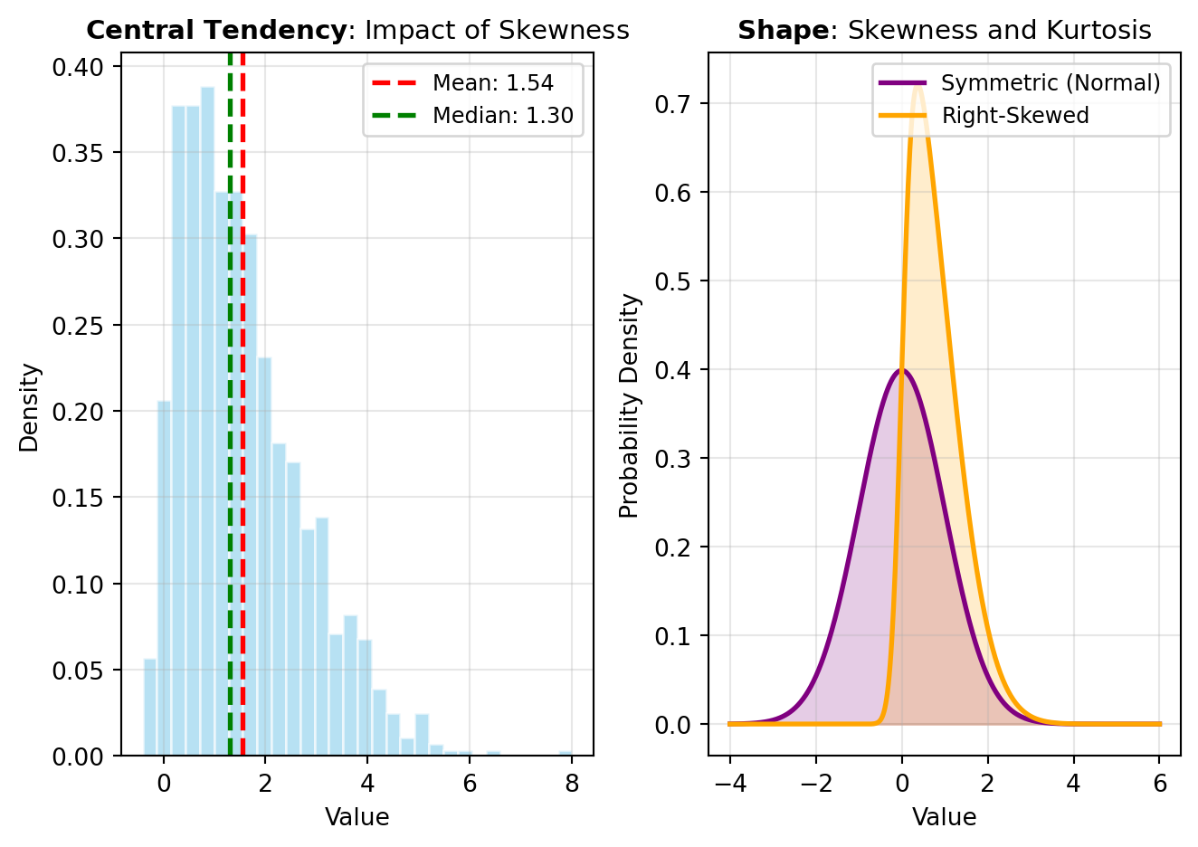
Central Tendency measures locate the “center” or typical value of a distribution. The most common include the mean (arithmetic average), median (middle value when sorted), and mode (most frequently occurring value). Each has distinct advantages: the mean leverages all data points but is sensitive to outliers, the median is robust to extreme values, and the mode identifies the most typical observation. Choosing the right central tendency measure depends on your data’s characteristics and analysis goals. For instance, DESCRIBE computes multiple central tendency statistics automatically, while MODE specifically isolates the most frequent value.

Dispersion measures quantify how spread out data points are around the center. Range, variance, and standard deviation capture different aspects of this spread. Variance measures the average squared deviation from the mean, while standard deviation is its square root, presented in the same units as the original data for easier interpretation. The interquartile range (IQR) represents the middle 50% of data, providing a robust alternative when outliers are present. Lower dispersion indicates data clusters tightly around the center; higher dispersion suggests greater variability. Understanding dispersion is critical because two datasets with identical means can have vastly different characteristics if their spreads differ.

Shape describes the distribution’s symmetry and peakedness. Skewness measures asymmetry: positive skew indicates a long tail extending right, while negative skew shows a tail extending left. Symmetric distributions have skewness near zero. Kurtosis measures the distribution’s tailedness—how peaked or flat it appears compared to a normal distribution. High kurtosis suggests heavy tails with extreme values; low kurtosis indicates lighter tails. These shape metrics reveal important distributional properties that central tendency and dispersion alone cannot capture.

Beyond standard moments, specialized averages serve specific purposes. The geometric mean (computed via GMEAN) is ideal for rates of change and data spanning multiple orders of magnitude. The harmonic mean (HMEAN) suits averaging rates and ratios. The power mean or generalized mean (PMEAN) unifies these concepts under a parameter-dependent framework. These alternatives to the arithmetic mean are implemented in NumPy and SciPy, Python’s fundamental libraries for numerical computing and scientific statistics.

Higher-order moments extend beyond simple statistics. The MOMENT function calculates arbitrary moments about the mean, providing flexibility for specialized analyses. The EXPECTILE function computes expectiles—a generalization of quantiles useful in risk analysis and asymmetric loss settings. For comparing groups, EFFECT_SIZES quantifies the magnitude of differences, crucial for interpreting statistical significance in applied contexts.

Figure 1: Summary Statistics in Distributions: (A) Central Tendency in Skewed Data—in symmetric distributions, mean and median align, while in right-skewed distributions, the mean is pulled toward the long tail. (B) Distribution Shape—comparing symmetric and right-skewed distributions reveals how skewness and kurtosis characterize distributional shape.

CRONBACH_ALPHA

This function estimates internal consistency reliability across multiple items intended to measure the same latent construct.

For k items with item variances \sigma_i^2 and total score variance \sigma_T^2, Cronbach’s alpha is:

\alpha = \frac{k}{k-1}\left(1 - \frac{\sum_{i=1}^{k}\sigma_i^2}{\sigma_T^2}\right)

Higher values indicate stronger internal consistency among items, subject to assumptions about dimensionality and measurement scale.

Excel Usage

=CRONBACH_ALPHA(data, items, scores, subject, cronbach_nan_policy)

data (list[list], required): Input table as a 2D range with a header row followed by data rows.
items (str, optional, default: null): Optional item identifier column for long-format data.
scores (str, optional, default: null): Optional score/value column for long-format data.
subject (str, optional, default: null): Optional subject identifier column for long-format data.
cronbach_nan_policy (str, optional, default: “pairwise”): Missing value handling strategy.

Returns (float): Cronbach’s alpha coefficient.

Example 1: Cronbach alpha from wide-format item matrix

Inputs:

data
i_one	i_two	i_three
3	4	3
4	4	5
2	3	2
5	5	4
4	3	4

Excel formula:

=CRONBACH_ALPHA({"i_one","i_two","i_three";3,4,3;4,4,5;2,3,2;5,5,4;4,3,4})

Expected output:

0.84

Example 2: Pairwise handling with missing cell in wide data

Inputs:

data			cronbach_nan_policy
i_one	i_two	i_three	pairwise
3	4	3
4		5
2	3	2
5	5	4
4	3	4

Excel formula:

=CRONBACH_ALPHA({"i_one","i_two","i_three";3,4,3;4,,5;2,3,2;5,5,4;4,3,4}, "pairwise")

Expected output:

0.850103

Example 3: Long-format table using subject, items, and scores

Inputs:

data			items	scores	subject
subj	item	score	item	score	subj
1	A	3
1	B	4
1	C	3
2	A	4
2	B	4
2	C	5
3	A	2
3	B	3
3	C	2
4	A	5
4	B	5
4	C	4

Excel formula:

=CRONBACH_ALPHA({"subj","item","score";1,"A",3;1,"B",4;1,"C",3;2,"A",4;2,"B",4;2,"C",5;3,"A",2;3,"B",3;3,"C",2;4,"A",5;4,"B",5;4,"C",4}, "item", "score", "subj")

Expected output:

0.9

Example 4: Long-format reliability with listwise policy

Inputs:

data			items	scores	subject	cronbach_nan_policy
subj	item	score	item	score	subj	listwise
1	A	3
1	B	4
1	C	3
2	A	4
2	B
2	C	5
3	A	2
3	B	3
3	C	2
4	A	5
4	B	5
4	C	4

Excel formula:

=CRONBACH_ALPHA({"subj","item","score";1,"A",3;1,"B",4;1,"C",3;2,"A",4;2,"B",;2,"C",5;3,"A",2;3,"B",3;3,"C",2;4,"A",5;4,"B",5;4,"C",4}, "item", "score", "subj", "listwise")

Expected output:

0.972973

Python Code

Show Code

import pandas as pd
import pingouin as pg

def cronbach_alpha(data, items=None, scores=None, subject=None, cronbach_nan_policy='pairwise'):
    """
    Compute Cronbach's alpha reliability coefficient for a set of items.

    See: https://pingouin-stats.org/generated/pingouin.cronbach_alpha.html

    This example function is provided as-is without any representation of accuracy.

    Args:
        data (list[list]): Input table as a 2D range with a header row followed by data rows.
        items (str, optional): Optional item identifier column for long-format data. Default is None.
        scores (str, optional): Optional score/value column for long-format data. Default is None.
        subject (str, optional): Optional subject identifier column for long-format data. Default is None.
        cronbach_nan_policy (str, optional): Missing value handling strategy. Valid options: Pairwise, Listwise. Default is 'pairwise'.

    Returns:
        float: Cronbach's alpha coefficient.
    """
    try:
        def to2d(value):
            return [[value]] if not isinstance(value, list) else value

        matrix = to2d(data)
        if not isinstance(matrix, list) or len(matrix) < 2 or not all(isinstance(row, list) for row in matrix):
            return "Error: Invalid input - data must be a 2D list with header and rows"

        headers = [str(col).strip() for col in matrix[0]]
        if len(headers) == 0 or any(col == "" for col in headers):
            return "Error: Invalid input - header row must contain non-empty column names"

        width = len(headers)
        records = []
        for row in matrix[1:]:
            values = list(row)
            if len(values) < width:
                values = values + [None] * (width - len(values))
            elif len(values) > width:
                values = values[:width]
            records.append(values)

        frame = pd.DataFrame(records, columns=headers)

        items_arg = None if items is None or str(items).strip() == "" else str(items)
        scores_arg = None if scores is None or str(scores).strip() == "" else str(scores)
        subject_arg = None if subject is None or str(subject).strip() == "" else str(subject)

        if (items_arg is None) != (scores_arg is None) or (items_arg is None) != (subject_arg is None):
            return "Error: Invalid input - items, scores, and subject must be provided together for long-format data"

        alpha_result = pg.cronbach_alpha(
            data=frame,
            items=items_arg,
            scores=scores_arg,
            subject=subject_arg,
            nan_policy=str(cronbach_nan_policy),
        )

        alpha_value = alpha_result[0] if isinstance(alpha_result, (list, tuple)) else alpha_result
        return float(alpha_value)
    except Exception as e:
        return f"Error: {str(e)}"

Online Calculator

data *

Input table as a 2D range with a header row followed by data rows.

items

Optional item identifier column for long-format data.

scores

Optional score/value column for long-format data.

subject

Optional subject identifier column for long-format data.

cronbach_nan_policy

Missing value handling strategy.

DESCRIBE

This function computes core descriptive statistics for a numeric dataset, including sample size, minimum, maximum, mean, variance, skewness, and kurtosis.

For observations x_1, x_2, \ldots, x_n, the reported mean and variance are based on:

\bar{x} = \frac{1}{n}\sum_{i=1}^{n} x_i, \quad s^2 = \frac{1}{n-\mathrm{ddof}}\sum_{i=1}^{n}(x_i-\bar{x})^2

The function flattens a 2D Excel range into one sample, ignores non-numeric entries, and returns all statistics in a single 2D row for spreadsheet output.

Excel Usage

=DESCRIBE(data, ddof, bias)

data (list[list], required): Table of numeric values to analyze.
ddof (int, optional, default: 0): Delta degrees of freedom for variance calculation.
bias (bool, optional, default: false): If True, calculations are not corrected for statistical bias.

Returns (list[list]): 2D list [[nobs, min, max, mean, var, skew, kurt]], or error string.

Example 1: Basic statistics with default parameters

Inputs:

data			ddof	bias
1	2	3	0	false
4	5	6

Excel formula:

=DESCRIBE({1,2,3;4,5,6}, 0, FALSE)

Expected output:

Result
6	1	6	3.5	2.91667	0	-1.2

Example 2: Statistics with ddof=1 for sample variance

Inputs:

data			ddof	bias
1	2	3	1	false
4	5	6

Excel formula:

=DESCRIBE({1,2,3;4,5,6}, 1, FALSE)

Expected output:

Result
6	1	6	3.5	3.5	0	-1.2

Example 3: Statistics with bias correction enabled

Inputs:

data			ddof	bias
1	2	3	0	true
4	5	6

Excel formula:

=DESCRIBE({1,2,3;4,5,6}, 0, TRUE)

Expected output:

Result
6	1	6	3.5	2.91667	0	-1.26857

Example 4: Statistics for larger values dataset

Inputs:

data			ddof	bias
10	20	30	0	false
40	50	60

Excel formula:

=DESCRIBE({10,20,30;40,50,60}, 0, FALSE)

Expected output:

Result
6	10	60	35	291.667	0	-1.2

Python Code

Show Code

import math
from scipy.stats import describe as scipy_describe

def describe(data, ddof=0, bias=False):
    """
    Compute descriptive statistics using scipy.stats.describe.

    See: https://docs.scipy.org/doc/scipy/reference/generated/scipy.stats.describe.html

    This example function is provided as-is without any representation of accuracy.

    Args:
        data (list[list]): Table of numeric values to analyze.
        ddof (int, optional): Delta degrees of freedom for variance calculation. Default is 0.
        bias (bool, optional): If True, calculations are not corrected for statistical bias. Default is False.

    Returns:
        list[list]: 2D list [[nobs, min, max, mean, var, skew, kurt]], or error string.
    """
    def to2d(x):
        return [[x]] if not isinstance(x, list) else x

    try:
      data = to2d(data)

      if not isinstance(data, list) or not all(isinstance(row, list) for row in data):
        return "Error: Invalid input: data must be a 2D list."

      flat = []
      for row in data:
        for x in row:
          try:
            val = float(x)
            if math.isfinite(val):
              flat.append(val)
          except (TypeError, ValueError):
            continue

      if len(flat) < 2:
        return "Error: Invalid input: data must contain at least two numeric values."

      if not isinstance(ddof, (int, float)) or int(ddof) != ddof or ddof < 0:
        return "Error: Invalid input: ddof must be a non-negative integer."

      if not isinstance(bias, bool):
        return "Error: Invalid input: bias must be a boolean."

      res = scipy_describe(flat, ddof=int(ddof), bias=bias)

      out = [
        int(res.nobs),
        float(res.minmax[0]),
        float(res.minmax[1]),
        float(res.mean),
        float(res.variance),
        float(res.skewness),
        float(res.kurtosis),
      ]
      return [out]
    except Exception as e:
      return f"Error: {str(e)}"

Online Calculator

data *

Table of numeric values to analyze.

ddof

Delta degrees of freedom for variance calculation.

bias

If True, calculations are not corrected for statistical bias.

DISTANCE_CORR

This function computes distance correlation, a dependence measure that detects both linear and non-linear associations between variables.

Distance correlation is zero if and only if the variables are independent (under finite first moments), making it more general than Pearson correlation for non-linear relationships.

The sample statistic is based on centered pairwise distance matrices and normalized distance covariance.

Excel Usage

=DISTANCE_CORR(x, y, n_boot, seed)

x (list[list], required): 2D range of numeric values for the first variable.
y (list[list], required): 2D range of numeric values for the second variable.
n_boot (int, optional, default: 0): Number of bootstrap samples for p-value estimation; set 0 to skip bootstrap.
seed (int, optional, default: null): Optional random seed for bootstrap reproducibility.

Returns (float): Distance correlation coefficient.

Example 1: Strong positive linear dependence

Inputs:

x	y
1	2
2	4
3	6
4	8
5	10
6	12

Excel formula:

=DISTANCE_CORR({1;2;3;4;5;6}, {2;4;6;8;10;12})

Expected output:

1

Example 2: Nonlinear monotonic dependence

Inputs:

x	y
1	1
2	4
3	9
4	16
5	25
6	36

Excel formula:

=DISTANCE_CORR({1;2;3;4;5;6}, {1;4;9;16;25;36})

Expected output:

0.98631

Example 3: Distance correlation with bootstrap setting

Inputs:

x	y	n_boot	seed
1	1	100	42
2	3
3	2
4	5
5	4
6	6

Excel formula:

=DISTANCE_CORR({1;2;3;4;5;6}, {1;3;2;5;4;6}, 100, 42)

Expected output:

0.884874

Example 4: Row vector inputs are flattened

Inputs:

x					y
1	2	3	4	5	5	4	3	2	1

Excel formula:

=DISTANCE_CORR({1,2,3,4,5}, {5,4,3,2,1})

Expected output:

1

Python Code

Show Code

import pingouin as pg

def distance_corr(x, y, n_boot=0, seed=None):
    """
    Compute distance correlation between two numeric variables.

    See: https://pingouin-stats.org/generated/pingouin.distance_corr.html

    This example function is provided as-is without any representation of accuracy.

    Args:
        x (list[list]): 2D range of numeric values for the first variable.
        y (list[list]): 2D range of numeric values for the second variable.
        n_boot (int, optional): Number of bootstrap samples for p-value estimation; set 0 to skip bootstrap. Default is 0.
        seed (int, optional): Optional random seed for bootstrap reproducibility. Default is None.

    Returns:
        float: Distance correlation coefficient.
    """
    try:
        def to2d(value):
            return [[value]] if not isinstance(value, list) else value

        def flatten_numeric(matrix):
            values = []
            for row in matrix:
                if not isinstance(row, list):
                    return None
                for item in row:
                    try:
                        values.append(float(item))
                    except (TypeError, ValueError):
                        continue
            return values

        x_matrix = to2d(x)
        y_matrix = to2d(y)

        if not isinstance(x_matrix, list) or not isinstance(y_matrix, list):
            return "Error: Invalid input - x and y must be 2D lists"

        x_values = flatten_numeric(x_matrix)
        y_values = flatten_numeric(y_matrix)
        if x_values is None or y_values is None:
            return "Error: Invalid input - x and y must be 2D lists"

        if len(x_values) != len(y_values):
            return "Error: Invalid input - x and y must contain the same number of numeric values"
        if len(x_values) < 2:
            return "Error: Invalid input - x and y must each contain at least two numeric values"

        seed_arg = None if seed is None else int(seed)
        n_boot_arg = None if int(n_boot) <= 0 else int(n_boot)

        result = pg.distance_corr(x_values, y_values, n_boot=n_boot_arg, seed=seed_arg)

        if isinstance(result, (tuple, list)):
            return float(result[0])
        return float(result)
    except Exception as e:
        return f"Error: {str(e)}"

Online Calculator

x *

2D range of numeric values for the first variable.

y *

2D range of numeric values for the second variable.

n_boot

Number of bootstrap samples for p-value estimation; set 0 to skip bootstrap.

seed

Optional random seed for bootstrap reproducibility.

EXPECTILE

This function computes an expectile at level \alpha for a numeric dataset, optionally using observation weights.

The expectile t is the solution of the asymmetric balance equation:

\alpha \sum_{i=1}^{n} w_i (x_i - t)_+ = (1-\alpha) \sum_{i=1}^{n} w_i (t - x_i)_+

where (u)_+ = \max(u, 0) and w_i=1 when no weights are supplied. At \alpha=0.5, the expectile equals the (weighted) mean.

Excel Usage

=EXPECTILE(data, alpha, weights)

data (list[list], required): A 2D column of numeric data.
alpha (float, optional, default: 0.5): The expectile to compute, a value between 0 and 1.
weights (list[list], optional, default: null): A 2D column of weights for each data point. Must have the same length as data.

Returns (float): The calculated expectile, or an error message (str) if input is invalid.

Example 1: Median expectile (alpha=0.5) without weights

Inputs:

data	alpha
1	0.5
2
3
4
5

Excel formula:

=EXPECTILE({1;2;3;4;5}, 0.5)

Expected output:

3

Example 2: Low alpha (0.2) expectile without weights

Inputs:

data	alpha
1	0.2
2
3
4
5

Excel formula:

=EXPECTILE({1;2;3;4;5}, 0.2)

Expected output:

2.18182

Example 3: High alpha (0.8) expectile with uniform weights

Inputs:

data	alpha	weights
1	0.8	1
2		1
3		1
4		1
5		1

Excel formula:

=EXPECTILE({1;2;3;4;5}, 0.8, {1;1;1;1;1})

Expected output:

3.81818

Example 4: Skewed weights emphasizing larger values

Inputs:

data	alpha	weights
1	0.5	1
2		1
3		1
4		1
10		4

Excel formula:

=EXPECTILE({1;2;3;4;10}, 0.5, {1;1;1;1;4})

Expected output:

6.25

Python Code

Show Code

from scipy.stats import expectile as scipy_expectile

def expectile(data, alpha=0.5, weights=None):
    """
    Calculates the expectile of a dataset using scipy.stats.expectile.

    See: https://docs.scipy.org/doc/scipy/reference/generated/scipy.stats.expectile.html

    This example function is provided as-is without any representation of accuracy.

    Args:
        data (list[list]): A 2D column of numeric data.
        alpha (float, optional): The expectile to compute, a value between 0 and 1. Default is 0.5.
        weights (list[list], optional): A 2D column of weights for each data point. Must have the same length as data. Default is None.

    Returns:
        float: The calculated expectile, or an error message (str) if input is invalid.
    """
    def to2d(x):
        return [[x]] if not isinstance(x, list) else x

    try:
      data = to2d(data)

      if not isinstance(data, list) or not all(isinstance(row, list) for row in data) or not data:
        return "Error: Invalid input: data must be a non-empty 2D list."

      a = []
      for row in data:
        for x in row:
          if not isinstance(x, (int, float)):
            return "Error: Invalid input: data must contain only numeric values."
          a.append(float(x))

      if not a:
        return "Error: Invalid input: data must contain at least one numeric value."

      if not isinstance(alpha, (int, float)):
        return "Error: Invalid input: alpha must be between 0 and 1."
      alpha = float(alpha)
      if not (0.0 <= alpha <= 1.0):
        return "Error: Invalid input: alpha must be between 0 and 1."

      w = None
      if weights is not None:
        weights = to2d(weights)
        if not isinstance(weights, list) or not all(isinstance(row, list) for row in weights):
          return "Error: Invalid input: weights must be a 2D list."

        flat_w = []
        for row in weights:
          for x in row:
            if not isinstance(x, (int, float)):
              return "Error: Invalid input: weights must contain only numeric values."
            if x < 0:
              return "Error: Invalid input: weights must be non-negative."
            flat_w.append(float(x))

        if len(flat_w) != len(a):
          return "Error: Invalid input: weights must have the same number of values as data."

        w = flat_w

      result = scipy_expectile(a=a, alpha=alpha, weights=w)
      return float(result)
    except Exception as e:
      return f"Error: {str(e)}"

Online Calculator

data *

A 2D column of numeric data.

alpha

The expectile to compute, a value between 0 and 1.

weights

A 2D column of weights for each data point. Must have the same length as data.

GMEAN

This function calculates the geometric mean of positive numeric values from a 2D input range.

For values x_1, x_2, \ldots, x_n with x_i > 0, the geometric mean is:

G = \left(\prod_{i=1}^{n} x_i\right)^{1/n}

Non-numeric values are ignored, and the function returns an error if no positive numeric values are available.

Excel Usage

=GMEAN(data)

data (list[list], required): 2D array of positive numeric values. Non-numeric values are ignored.

Returns (float): Geometric mean of the input data, or error message (str) if input is invalid.

Example 1: Geometric mean of 2x2 matrix

Inputs:

data
1	2
3	4

Excel formula:

=GMEAN({1,2;3,4})

Expected output:

2.21336

Example 2: Non-numeric values are ignored

Inputs:

data
2	a
8	4

Excel formula:

=GMEAN({2,"a";8,4})

Expected output:

4

Example 3: Single row of values

Inputs:

data
5	10

Excel formula:

=GMEAN({5,10})

Expected output:

7.07107

Example 4: Single column with multiple rows

Inputs:

data
2
8
32

Excel formula:

=GMEAN({2;8;32})

Expected output:

8

Python Code

Show Code

from scipy.stats import gmean as scipy_gmean

def gmean(data):
    """
    Compute the geometric mean of the input data, flattening the input and ignoring non-numeric values.

    See: https://docs.scipy.org/doc/scipy/reference/generated/scipy.stats.gmean.html

    This example function is provided as-is without any representation of accuracy.

    Args:
        data (list[list]): 2D array of positive numeric values. Non-numeric values are ignored.

    Returns:
        float: Geometric mean of the input data, or error message (str) if input is invalid.
    """
    def to2d(x):
        return [[x]] if not isinstance(x, list) else x

    try:
      data = to2d(data)

      if not isinstance(data, list) or not all(isinstance(row, list) for row in data):
        return "Error: Invalid input: data must be a 2D list."

      flat = []
      for row in data:
        for x in row:
          try:
            val = float(x)
            if val > 0:
              flat.append(val)
          except (TypeError, ValueError):
            continue

      if not flat:
        return "Error: Input must contain at least one positive number."

      result = scipy_gmean(flat)
      return float(result)
    except Exception as e:
      return f"Error: {str(e)}"

Online Calculator

data *

2D array of positive numeric values. Non-numeric values are ignored.

HMEAN

This function computes the harmonic mean of positive numeric values in a 2D input range.

For values x_1, x_2, \ldots, x_n with x_i > 0, the harmonic mean is:

H = \frac{n}{\sum_{i=1}^{n} \frac{1}{x_i}}

The harmonic mean emphasizes smaller values and is commonly used for rates and ratios. Non-numeric entries are ignored, and at least one positive value is required.

Excel Usage

=HMEAN(data)

data (list[list], required): 2D array of positive numeric values. Non-numeric values are ignored.

Returns (float): Harmonic mean of the input data, or error message (str) if input is invalid.

Example 1: Harmonic mean of 2x2 matrix

Inputs:

data
1	2
3	4

Excel formula:

=HMEAN({1,2;3,4})

Expected output:

1.92

Example 2: Single column with multiple rows

Inputs:

data
2
4
8
16

Excel formula:

=HMEAN({2;4;8;16})

Expected output:

4.26667

Example 3: Non-numeric values are ignored

Inputs:

data
5	6
text	7

Excel formula:

=HMEAN({5,6;"text",7})

Expected output:

5.88785

Example 4: Harmonic mean of 3x2 matrix

Inputs:

data
10	20	30
40	50	60

Excel formula:

=HMEAN({10,20,30;40,50,60})

Expected output:

24.4898

Python Code

Show Code

from scipy.stats import hmean as scipy_hmean

def hmean(data):
    """
    Calculates the harmonic mean of the input data, flattening the input and ignoring non-numeric values.

    See: https://docs.scipy.org/doc/scipy/reference/generated/scipy.stats.hmean.html

    This example function is provided as-is without any representation of accuracy.

    Args:
        data (list[list]): 2D array of positive numeric values. Non-numeric values are ignored.

    Returns:
        float: Harmonic mean of the input data, or error message (str) if input is invalid.
    """
    def to2d(x):
        return [[x]] if not isinstance(x, list) else x

    try:
      data = to2d(data)

      if not isinstance(data, list) or not all(isinstance(row, list) for row in data):
        return "Error: Invalid input: data must be a 2D list."

      flat = []
      for row in data:
        for item in row:
          try:
            val = float(item)
            if val > 0:
              flat.append(val)
          except (TypeError, ValueError):
            continue

      if not flat:
        return "Error: Input must contain at least one positive number."

      result = scipy_hmean(flat)
      return float(result)
    except Exception as e:
      return f"Error: {str(e)}"

Online Calculator

data *

2D array of positive numeric values. Non-numeric values are ignored.

KURTOSIS

This function measures tail heaviness and peakedness of a distribution using sample kurtosis.

If m_2 and m_4 are the second and fourth central moments,

ext{Pearson kurtosis} = \frac{m_4}{m_2^2}, \quad ext{Fisher kurtosis} = \frac{m_4}{m_2^2} - 3

Setting fisher=true returns the excess kurtosis (normal distribution near 0), while fisher=false returns Pearson kurtosis (normal distribution near 3).

Excel Usage

=KURTOSIS(data, fisher, bias)

data (list[list], required): 2D array of numeric values. Non-numeric values are ignored.
fisher (bool, optional, default: true): If True, Fisher’s definition is used (normal ==> 0.0). If False, Pearson’s definition is used (normal ==> 3.0).
bias (bool, optional, default: true): If False, calculations are corrected for statistical bias.

Returns (float): Kurtosis of the data, or error message (str) if input is invalid.

Example 1: Fisher kurtosis with bias (default)

Inputs:

data
1
2
3
4

Excel formula:

=KURTOSIS({1;2;3;4})

Expected output:

-1.36

Example 2: Pearson kurtosis with bias

Inputs:

data	fisher
1	false
2
3
4

Excel formula:

=KURTOSIS({1;2;3;4}, FALSE)

Expected output:

1.64

Example 3: Fisher kurtosis with bias correction

Inputs:

data	fisher	bias
1	true	false
2
3
4

Excel formula:

=KURTOSIS({1;2;3;4}, TRUE, FALSE)

Expected output:

-1.2

Example 4: Pearson kurtosis with bias correction

Inputs:

data	fisher	bias
1	false	false
2
3
4

Excel formula:

=KURTOSIS({1;2;3;4}, FALSE, FALSE)

Expected output:

1.8

Python Code

Show Code

from scipy.stats import kurtosis as scipy_kurtosis

def kurtosis(data, fisher=True, bias=True):
    """
    Compute the kurtosis (Fisher or Pearson) of a dataset.

    See: https://docs.scipy.org/doc/scipy/reference/generated/scipy.stats.kurtosis.html

    This example function is provided as-is without any representation of accuracy.

    Args:
        data (list[list]): 2D array of numeric values. Non-numeric values are ignored.
        fisher (bool, optional): If True, Fisher's definition is used (normal ==> 0.0). If False, Pearson's definition is used (normal ==> 3.0). Default is True.
        bias (bool, optional): If False, calculations are corrected for statistical bias. Default is True.

    Returns:
        float: Kurtosis of the data, or error message (str) if input is invalid.
    """
    def to2d(x):
        return [[x]] if not isinstance(x, list) else x

    try:
      data = to2d(data)

      if not isinstance(data, list) or not all(isinstance(row, list) for row in data):
        return "Error: Invalid input: data must be a 2D list."

      if not isinstance(fisher, bool):
        return "Error: Invalid input: fisher must be a boolean."

      if not isinstance(bias, bool):
        return "Error: Invalid input: bias must be a boolean."

      flat = []
      for row in data:
        for x in row:
          try:
            val = float(x)
            flat.append(val)
          except (TypeError, ValueError):
            continue

      if len(flat) < 2:
        return "Error: Invalid input: data must contain at least two numeric values."

      result = scipy_kurtosis(flat, fisher=fisher, bias=bias, nan_policy='omit')
      return float(result)
    except Exception as e:
      return f"Error: {str(e)}"

Online Calculator

data *

2D array of numeric values. Non-numeric values are ignored.

fisher

If True, Fisher's definition is used (normal ==> 0.0). If False, Pearson's definition is used (normal ==> 3.0).

bias

If False, calculations are corrected for statistical bias.

MODE

This function returns the mode, the most frequently occurring numeric value, from a 2D dataset.

For frequency counts f(v) over unique values v, the mode is any value maximizing frequency:

v_{\text{mode}} \in \arg\max_{v} f(v)

In this wrapper, non-numeric cells are ignored and an error is returned when no value repeats (that is, when no mode exists under the selected rule).

Excel Usage

=MODE(data)

data (list[list], required): 2D array of numeric values to find the mode of. Non-numeric values are ignored.

Returns (float): The most common value in the data, or str error message if invalid.

Example 1: Simple mode with repeated value

Inputs:

data
1	2
2	3
2	4

Excel formula:

=MODE({1,2;2,3;2,4})

Expected output:

2

Example 2: Multiple modes returns smallest

Inputs:

data
1	2
2	1
3	3

Excel formula:

=MODE({1,2;2,1;3,3})

Expected output:

1

Example 3: Non-numeric values ignored

Inputs:

data
1	a
2	2
2	b

Excel formula:

=MODE({1,"a";2,2;2,"b"})

Expected output:

2

Example 4: Mode of a larger array

Inputs:

data
10	20	30
20	40	50
60	20	80

Excel formula:

=MODE({10,20,30;20,40,50;60,20,80})

Expected output:

20

Python Code

Show Code

from scipy.stats import mode as scipy_mode

def mode(data):
    """
    Return the modal (most common) numeric value in the input data, returning the smallest if there are multiple modes.

    See: https://docs.scipy.org/doc/scipy/reference/generated/scipy.stats.mode.html

    This example function is provided as-is without any representation of accuracy.

    Args:
        data (list[list]): 2D array of numeric values to find the mode of. Non-numeric values are ignored.

    Returns:
        float: The most common value in the data, or str error message if invalid.
    """
    # Helper function to normalize scalar input to 2D list
    def to2d(x):
        return [[x]] if not isinstance(x, list) else x

    try:
      # Normalize input for 2D list args
      data = to2d(data)

      # If input is not a list of lists, return error
      if not isinstance(data, list) or not all(isinstance(row, list) for row in data):
        return "Error: Invalid input: data must be a 2D list."
      # Flatten and filter numeric values
      flat = []
      for row in data:
        for val in row:
          try:
            v = float(val)
            flat.append(v)
          except (ValueError, TypeError):
            continue
      if len(flat) < 2:
        return "Error: Invalid input: data must contain at least two numeric values."
      # Use scipy.stats.mode
      res = scipy_mode(flat, keepdims=False, axis=None, nan_policy='omit')
      if res.count < 2:
        return "Error: No mode found. At least one value must appear more than once."
      # Return as Python float scalar, not numpy type
      mode_value = float(res.mode.item()) if hasattr(res.mode, 'item') else float(res.mode)
      return mode_value
    except Exception as e:
      return f"Error: {str(e)}"

Online Calculator

data *

2D array of numeric values to find the mode of. Non-numeric values are ignored.

MOMENT

This function computes the central moment of specified integer order for numeric data.

For observations x_1, \ldots, x_n with mean \bar{x}, the order-k central moment is:

m_k = \frac{1}{n}\sum_{i=1}^{n}(x_i-\bar{x})^k

Lower moments describe key distribution shape features: order 2 relates to spread, order 3 to asymmetry, and order 4 to tail behavior.

Excel Usage

=MOMENT(data, order)

data (list[list], required): 2D array of numeric values. Non-numeric values are ignored.
order (int, required): Order of the moment to calculate (must be a positive integer).

Returns (float): The nth moment about the mean, or error message (str) if input is invalid.

Example 1: Second moment (variance) of a column vector

Inputs:

data	order
1	2
2
3
4
5

Excel formula:

=MOMENT({1;2;3;4;5}, 2)

Expected output:

2

Example 2: Third moment (skewness) of a row vector

Inputs:

data					order
1	2	3	4	5	3

Excel formula:

=MOMENT({1,2,3,4,5}, 3)

Expected output:

0

Example 3: Fourth moment (kurtosis) of a matrix

Inputs:

data			order
1	2	3	4
4	5	6

Excel formula:

=MOMENT({1,2,3;4,5,6}, 4)

Expected output:

14.7292

Example 4: First moment of a column vector (always zero)

Inputs:

data	order
10	1
20
30

Excel formula:

=MOMENT({10;20;30}, 1)

Expected output:

0

Python Code

Show Code

from scipy.stats import moment as scipy_moment
import math

def moment(data, order):
    """
    Calculates the nth moment about the mean for a sample.

    See: https://docs.scipy.org/doc/scipy/reference/generated/scipy.stats.moment.html

    This example function is provided as-is without any representation of accuracy.

    Args:
        data (list[list]): 2D array of numeric values. Non-numeric values are ignored.
        order (int): Order of the moment to calculate (must be a positive integer).

    Returns:
        float: The nth moment about the mean, or error message (str) if input is invalid.
    """
    def to2d(x):
        return [[x]] if not isinstance(x, list) else x

    try:
      data = to2d(data)

      if not isinstance(data, list) or not all(isinstance(row, list) for row in data):
        return "Error: Invalid input: data must be a 2D list."

      flat = []
      for row in data:
        for x in row:
          try:
            val = float(x)
            if math.isfinite(val):
              flat.append(val)
          except (TypeError, ValueError):
            continue

      if len(flat) < 2:
        return "Error: Invalid input: data must contain at least two numeric values."

      if not isinstance(order, (int, float)) or int(order) != order or order < 1:
        return "Error: Invalid input: order must be a positive integer."

      result = scipy_moment(flat, order=int(order), axis=None, nan_policy='omit')
      return float(result)
    except Exception as e:
      return f"Error: {str(e)}"

Online Calculator

data *

2D array of numeric values. Non-numeric values are ignored.

order *

Order of the moment to calculate (must be a positive integer).

PARTIAL_CORR

This function measures the association between two variables while controlling for one or more covariates.

For variables X and Y adjusted for covariates Z, the partial correlation is the correlation between residuals:

r_{XY\cdot Z} = \mathrm{corr}(\varepsilon_X, \varepsilon_Y)

where \varepsilon_X and \varepsilon_Y are residuals after regressing X and Y on Z. This can isolate direct linear or rank-based association from confounding effects.

Excel Usage

=PARTIAL_CORR(data, x, y, covar, x_covar, y_covar, pcorr_method, pcorr_alternative)

data (list[list], required): Input table as a 2D range with a header row followed by data rows.
x (str, required): Name of the first variable column.
y (str, required): Name of the second variable column.
covar (str, optional, default: null): Optional covariate name or comma-separated covariate names.
x_covar (str, optional, default: null): Optional covariates to control only in x (comma-separated names).
y_covar (str, optional, default: null): Optional covariates to control only in y (comma-separated names).
pcorr_method (str, optional, default: “pearson”): Correlation method.
pcorr_alternative (str, optional, default: “two-sided”): Alternative hypothesis for the p-value computation.

Returns (float): Partial correlation coefficient r.

Example 1: Partial correlation controlling one covariate

Inputs:

data			x	y	covar
x	y	z	x	y	z
1	2	0
2	3	1
3	5	1
4	4	2
5	7	3
6	8	3

Excel formula:

=PARTIAL_CORR({"x","y","z";1,2,0;2,3,1;3,5,1;4,4,2;5,7,3;6,8,3}, "x", "y", "z")

Expected output:

0.673891

Example 2: Semi-partial using x_covar only

Inputs:

data			x	y	x_covar	pcorr_method
x	y	z	x	y	z	spearman
1	3	1
2	3	1
3	4	2
4	6	3
5	7	3
6	9	4

Excel formula:

=PARTIAL_CORR({"x","y","z";1,3,1;2,3,1;3,4,2;4,6,3;5,7,3;6,9,4}, "x", "y", "z", "spearman")

Expected output:

0.121268

Example 3: Multiple covariates as comma-separated names

Inputs:

data				x	y	covar
x	y	z1	z2	x	y	z1, z2
1	2	0	1
2	3	1	2
3	5	1	3
4	4	2	2
5	7	3	5
6	8	3	6

Excel formula:

=PARTIAL_CORR({"x","y","z1","z2";1,2,0,1;2,3,1,2;3,5,1,3;4,4,2,2;5,7,3,5;6,8,3,6}, "x", "y", "z1, z2")

Expected output:

0.727688

Example 4: Partial correlation with one-sided alternative

Inputs:

data			x	y	covar	pcorr_alternative
x	y	z	x	y	z	greater
1	2	1
2	4	1
3	6	2
4	7	2
5	9	3
6	11	3

Excel formula:

=PARTIAL_CORR({"x","y","z";1,2,1;2,4,1;3,6,2;4,7,2;5,9,3;6,11,3}, "x", "y", "z", "greater")

Expected output:

0.96225

Python Code

Show Code

import pandas as pd
import pingouin as pg

def partial_corr(data, x, y, covar=None, x_covar=None, y_covar=None, pcorr_method='pearson', pcorr_alternative='two-sided'):
    """
    Compute partial or semi-partial correlation between two variables.

    See: https://pingouin-stats.org/generated/pingouin.partial_corr.html

    This example function is provided as-is without any representation of accuracy.

    Args:
        data (list[list]): Input table as a 2D range with a header row followed by data rows.
        x (str): Name of the first variable column.
        y (str): Name of the second variable column.
        covar (str, optional): Optional covariate name or comma-separated covariate names. Default is None.
        x_covar (str, optional): Optional covariates to control only in x (comma-separated names). Default is None.
        y_covar (str, optional): Optional covariates to control only in y (comma-separated names). Default is None.
        pcorr_method (str, optional): Correlation method. Valid options: Pearson, Spearman. Default is 'pearson'.
        pcorr_alternative (str, optional): Alternative hypothesis for the p-value computation. Valid options: Two-sided, Less, Greater. Default is 'two-sided'.

    Returns:
        float: Partial correlation coefficient r.
    """
    try:
        def to2d(value):
            return [[value]] if not isinstance(value, list) else value

        def parse_names(value):
            if value is None:
                return None
            text = str(value).strip()
            if text == "":
                return None
            names = [part.strip() for part in text.split(",") if part.strip()]
            if len(names) == 0:
                return None
            return names if len(names) > 1 else names[0]

        matrix = to2d(data)
        if not isinstance(matrix, list) or len(matrix) < 2 or not all(isinstance(row, list) for row in matrix):
            return "Error: Invalid input - data must be a 2D list with header and rows"

        headers = [str(col).strip() for col in matrix[0]]
        if len(headers) == 0 or any(col == "" for col in headers):
            return "Error: Invalid input - header row must contain non-empty column names"

        width = len(headers)
        records = []
        for row in matrix[1:]:
            values = list(row)
            if len(values) < width:
                values = values + [None] * (width - len(values))
            elif len(values) > width:
                values = values[:width]
            records.append(values)

        frame = pd.DataFrame(records, columns=headers)

        covar_arg = parse_names(covar)
        x_covar_arg = parse_names(x_covar)
        y_covar_arg = parse_names(y_covar)

        if covar_arg is None and x_covar_arg is None and y_covar_arg is None:
            return "Error: Invalid input - provide covar, x_covar, or y_covar"
        if covar_arg is not None and (x_covar_arg is not None or y_covar_arg is not None):
            return "Error: Invalid input - use covar or x_covar/y_covar, not both"

        result = pg.partial_corr(
            data=frame,
            x=str(x),
            y=str(y),
            covar=covar_arg,
            x_covar=x_covar_arg,
            y_covar=y_covar_arg,
            method=str(pcorr_method),
            alternative=str(pcorr_alternative),
        )

        if "r" not in result.columns or len(result.index) == 0:
            return "Error: Unable to compute partial correlation"

        return float(result.loc[result.index[0], "r"])
    except Exception as e:
        return f"Error: {str(e)}"

Online Calculator

data *

Input table as a 2D range with a header row followed by data rows.

x *

Name of the first variable column.

y *

Name of the second variable column.

covar

Optional covariate name or comma-separated covariate names.

x_covar

Optional covariates to control only in x (comma-separated names).

y_covar

Optional covariates to control only in y (comma-separated names).

pcorr_method

Correlation method.

pcorr_alternative

Alternative hypothesis for the p-value computation.

PMEAN

This function computes the generalized (power) mean of positive numeric data for exponent p.

For values x_1, x_2, \ldots, x_n, the power mean is:

M_p = \left(\frac{1}{n}\sum_{i=1}^{n} x_i^p\right)^{1/p}

Special cases include arithmetic mean (p=1), geometric mean as the limit at p \to 0, and harmonic mean (p=-1).

Excel Usage

=PMEAN(data, p)

data (list[list], required): 2D array of numeric values. Non-numeric values are ignored.
p (float, required): The power exponent for the generalized mean (e.g., 1 for arithmetic, 0 for geometric, -1 for harmonic).

Returns (float): Power mean (float), or error message string.

Example 1: Arithmetic mean (p=1)

Inputs:

data		p
1	2	1
3	4

Excel formula:

=PMEAN({1,2;3,4}, 1)

Expected output:

2.5

Example 2: Geometric mean (p=0)

Inputs:

data		p
1	2	0
3	4

Excel formula:

=PMEAN({1,2;3,4}, 0)

Expected output:

2.21336

Example 3: Harmonic mean (p=-1)

Inputs:

data		p
1	2	-1
3	4

Excel formula:

=PMEAN({1,2;3,4}, -1)

Expected output:

1.92

Example 4: Quadratic mean (p=2)

Inputs:

data		p
1	2	2
3	4

Excel formula:

=PMEAN({1,2;3,4}, 2)

Expected output:

2.73861

Python Code

Show Code

import math
from scipy.stats import pmean as scipy_pmean

def pmean(data, p):
    """
    Computes the power mean (generalized mean) of the input data for a given power p.

    See: https://docs.scipy.org/doc/scipy/reference/generated/scipy.stats.pmean.html

    This example function is provided as-is without any representation of accuracy.

    Args:
        data (list[list]): 2D array of numeric values. Non-numeric values are ignored.
        p (float): The power exponent for the generalized mean (e.g., 1 for arithmetic, 0 for geometric, -1 for harmonic).

    Returns:
        float: Power mean (float), or error message string.
    """
    def to2d(x):
        return [[x]] if not isinstance(x, list) else x

    try:
      data = to2d(data)

      if not isinstance(data, list) or not all(isinstance(row, list) for row in data):
        return "Error: Invalid input: data must be a 2D list."

      flat = []
      for row in data:
        for val in row:
          try:
            v = float(val)
            if math.isfinite(v):
              flat.append(v)
          except (ValueError, TypeError):
            continue

      if not flat:
        return "Error: Invalid input: data must contain at least one numeric value."

      if not isinstance(p, (int, float)):
        return "Error: Invalid input: p must be a number."

      p = float(p)
      if not math.isfinite(p):
        return "Error: Invalid input: p must be a finite number."

      for v in flat:
        if v <= 0:
          return "Error: Invalid input: all values must be positive."

      result = scipy_pmean(flat, p, axis=None, nan_policy='omit', keepdims=False)
      return float(result)
    except Exception as e:
      return f"Error: {str(e)}"

Online Calculator

data *

2D array of numeric values. Non-numeric values are ignored.

p *

The power exponent for the generalized mean (e.g., 1 for arithmetic, 0 for geometric, -1 for harmonic).

SKEWNESS

This function measures distribution asymmetry using sample skewness.

Using central moments m_2 and m_3, the Fisher-Pearson skewness coefficient is:

g_1 = \frac{m_3}{m_2^{3/2}}

Positive skewness indicates a longer right tail, negative skewness indicates a longer left tail, and values near zero suggest approximate symmetry.

Excel Usage

=SKEWNESS(data, bias)

data (list[list], required): 2D array of numeric values. Non-numeric values are ignored.
bias (bool, optional, default: true): If True, calculations are not corrected for statistical bias.

Returns (float): Skewness value (float), or error message string.

Example 1: Right skewed data returns positive skewness

Inputs:

data	bias
1	true
2
3
4
10

Excel formula:

=SKEWNESS({1;2;3;4;10}, TRUE)

Expected output:

1.13842

Example 2: Left skewed data returns negative skewness

Inputs:

data	bias
1	true
7
8
9
10

Excel formula:

=SKEWNESS({1;7;8;9;10}, TRUE)

Expected output:

-1.13842

Example 3: Symmetric data returns zero skewness (biased)

Inputs:

data	bias
1	true
2
3
4
5

Excel formula:

=SKEWNESS({1;2;3;4;5}, TRUE)

Expected output:

0

Example 4: Symmetric data returns zero skewness (unbiased)

Inputs:

data	bias
1	false
2
3
4
5

Excel formula:

=SKEWNESS({1;2;3;4;5}, FALSE)

Expected output:

0

Python Code

Show Code

import math
from scipy.stats import skew as scipy_skew

def skewness(data, bias=True):
    """
    Calculate the skewness of a dataset.

    See: https://docs.scipy.org/doc/scipy/reference/generated/scipy.stats.skew.html

    This example function is provided as-is without any representation of accuracy.

    Args:
        data (list[list]): 2D array of numeric values. Non-numeric values are ignored.
        bias (bool, optional): If True, calculations are not corrected for statistical bias. Default is True.

    Returns:
        float: Skewness value (float), or error message string.
    """
    def to2d(x):
        return [[x]] if not isinstance(x, list) else x

    try:
      data = to2d(data)

      if not isinstance(data, list) or not all(isinstance(row, list) for row in data) or not data:
        return "Error: Invalid input: data must be a non-empty 2D list."

      if not isinstance(bias, bool):
        return "Error: Invalid input: bias must be a boolean."

      flat_data = []
      for row in data:
        for item in row:
          try:
            val = float(item)
            if math.isfinite(val):
              flat_data.append(val)
          except (ValueError, TypeError):
            continue

      if len(flat_data) < 3 and not bias:
        return "Error: Invalid input: At least 3 data points are required for unbiased skewness calculation."
      if len(flat_data) < 2:
        return "Error: Invalid input: At least 2 data points are required for skewness calculation."

      result = scipy_skew(flat_data, bias=bias)

      return float(result)
    except Exception as e:
      return f"Error: {str(e)}"

Online Calculator

data *

2D array of numeric values. Non-numeric values are ignored.

bias

If True, calculations are not corrected for statistical bias.